规模法则

Prof. Benjamin Widom accepted the invitation on 4 February 2009 (self-imposed deadline: 4 August 2009).

http://www.scholarpedia.org/w/index.php?title=Scaling_laws&action=edit https://imagej.nih.gov/ij/plugins/fraclac/FLHelp/Glossary.htm#scalingrulemmt

Scaling laws are the expression of physical principles in the mathematical language of homogeneous functions.

标度律是物理原理在齐次函数数学语言中的表达。

Introduction 引言

A function [math]\displaystyle{ f (x, y, z,\ldots) }[/math] is said to be homogeneous of degree [math]\displaystyle{ n }[/math] in the variables [math]\displaystyle{ x,y,z,\ldots }[/math] if, identically for all [math]\displaystyle{ \lambda\ , }[/math]

[math]\displaystyle{ \label{eq:1} f(\lambda x, \lambda y, \lambda z, \ldots) \equiv \lambda^{n}f (x, y, z, \ldots). }[/math]

如果对所有[math]\displaystyle{ \lambda\ }[/math]都满足关系

[math]\displaystyle{ f(\lambda x, \lambda y, \lambda z, \ldots) \equiv \lambda^{n}f (x, y, z, \ldots). }[/math]

(1)

则称函数[math]\displaystyle{ f (x, y, z,\ldots) }[/math]是变量[math]\displaystyle{ x,y,z,\ldots }[/math]的[math]\displaystyle{ n }[/math]次齐次函数。

For example, [math]\displaystyle{ ax^2 + bxy + cy^2 }[/math] is homogeneous of degree 2 in [math]\displaystyle{ x }[/math] and [math]\displaystyle{ y }[/math] and of the first degree in [math]\displaystyle{ a, b, }[/math] and [math]\displaystyle{ c\ . }[/math]

例如，[math]\displaystyle{ ax^2 + bxy + cy^2 }[/math]是[math]\displaystyle{ x }[/math]和[math]\displaystyle{ y }[/math]二次齐次函数，而对[math]\displaystyle{ a, b, }[/math][math]\displaystyle{ c\ }[/math]则是一次齐次。

By setting [math]\displaystyle{ \lambda = 1/x }[/math] in (1) we have as an alternative expression of homogeneity: [math]\displaystyle{ f (x, y, z, \ldots) }[/math] is homogeneous of degree [math]\displaystyle{ n }[/math] in [math]\displaystyle{ x, y, z, \ldots }[/math] if

[math]\displaystyle{ \label{eq:2} f(x, y, z, \ldots) = x^nf(1, y/x, z/x, \ldots) \equiv x^n\phi(y/x, z/x, \ldots); }[/math]

将[math]\displaystyle{ \lambda = 1/x }[/math]带入(1)，则有齐次性的另一种表达式，如果[math]\displaystyle{ f (x, y, z, \ldots) }[/math]满足关系：

[math]\displaystyle{ f(x, y, z, \ldots) = x^nf(1, y/x, z/x, \ldots) \equiv x^n\phi(y/x, z/x, \ldots); }[/math]

(2)

则它是[math]\displaystyle{ x, y, z, \ldots }[/math]的[math]\displaystyle{ n }[/math]次齐次函数。

i.e., the [math]\displaystyle{ n^{th} }[/math] power of [math]\displaystyle{ x }[/math] times some function [math]\displaystyle{ \phi }[/math] of the ratios [math]\displaystyle{ y/x, z/x, \ldots }[/math] alone.

If [math]\displaystyle{ f (x, y, z, \ldots) }[/math] is homogeneous of degree [math]\displaystyle{ n }[/math] in [math]\displaystyle{ x, y, z, \ldots }[/math] it satisfies Euler's theorem :

[math]\displaystyle{ \label{eq:3} x\frac{\partial f}{\partial x}+y\frac{\partial f}{\partial y}+z\frac{\partial f}{\partial z}+\cdots \equiv nf. }[/math]

如果[math]\displaystyle{ f (x, y, z, \ldots) }[/math]对[math]\displaystyle{ x, y, z, \ldots }[/math]是[math]\displaystyle{ n }[/math]次齐次的，则它满足欧拉定理：

[math]\displaystyle{ x\frac{\partial f}{\partial x}+y\frac{\partial f}{\partial y}+z\frac{\partial f}{\partial z}+\cdots \equiv nf. }[/math]

(3)

In thermodynamics, if the scale of a system is merely increased by a factor [math]\displaystyle{ \lambda }[/math] with no change in its intensive properties, then all its extensive properties including its entropy [math]\displaystyle{ S\ , }[/math] energy [math]\displaystyle{ E\ , }[/math] volume [math]\displaystyle{ V\ , }[/math] and the masses [math]\displaystyle{ m_1, m_2, \ldots }[/math] of each of its chemical constituents are increased by that factor, so the extensive function [math]\displaystyle{ S(E, V, m_1, m_2, \ldots) }[/math] is homogeneous of degree 1 in its extensive arguments:

[math]\displaystyle{ \label{eq:4} S(\lambda E, \lambda V, \lambda {m_1}, \lambda {m_2}, \ldots ) = \lambda S(E, V, {m_1}, {m_2}, \ldots). }[/math]

在热力学 Thermodynamics中，如果一个系统的标度增加[math]\displaystyle{ \lambda }[/math]倍而其强度量不发生变化，则该系统所有化学组分的广度量（如熵[math]\displaystyle{ S\ , }[/math]能量[math]\displaystyle{ E\ , }[/math]体积[math]\displaystyle{ V\ , }[/math]质量[math]\displaystyle{ m_1, m_2, \ldots }[/math]等）也增加相同倍数。因此广度函数[math]\displaystyle{ S(E, V, m_1, m_2, \ldots) }[/math]在广义论证中满足齐次关系：

[math]\displaystyle{ S(\lambda E, \lambda V, \lambda {m_1}, \lambda {m_2}, \ldots ) = \lambda S(E, V, {m_1}, {m_2}, \ldots). }[/math]

(4)

With [math]\displaystyle{ T }[/math] the temperature, [math]\displaystyle{ p }[/math] the pressure, and [math]\displaystyle{ \mu_i }[/math] the chemical potential of the species [math]\displaystyle{ i\ , }[/math] we have the thermodynamic relations [math]\displaystyle{ \partial S/\partial E = 1/T\ , }[/math] [math]\displaystyle{ \partial S/\partial V = p/T\ , }[/math] and [math]\displaystyle{ \partial S/\partial m_i = - \mu_i/T\ ; }[/math] so from Euler's theorem,

[math]\displaystyle{ \label{eq:5} \frac{1}{T} (E + pV - \mu_1m_1 - \mu_2m_2 - \cdots) =S, }[/math]

以[math]\displaystyle{ T }[/math]，[math]\displaystyle{ p }[/math]，[math]\displaystyle{ \mu_i }[/math] 分别表示温度，压力和不同组分[math]\displaystyle{ i\ }[/math]的化学势，根据热力学关系 [math]\displaystyle{ \partial S/\partial E = 1/T\ , }[/math] [math]\displaystyle{ \partial S/\partial V = p/T\ , }[/math] 和[math]\displaystyle{ \partial S/\partial m_i = - \mu_i/T\ ; }[/math]再由欧拉定理可得：

[math]\displaystyle{ \frac{1}{T} (E + pV - \mu_1m_1 - \mu_2m_2 - \cdots) =S, }[/math]

(5)

an important identity. Any extensive function [math]\displaystyle{ X(T, p, m_1, m_2, \ldots)\ , }[/math] such as the volume V or the Gibbs free energy [math]\displaystyle{ E+pV-TS\ , }[/math] is homogeneous of the first degree in the [math]\displaystyle{ m_i }[/math] at fixed [math]\displaystyle{ p }[/math] and [math]\displaystyle{ T\ , }[/math] so

[math]\displaystyle{ \label{eq:6} X = m_1 \frac{\partial X}{\partial m_1} + m_2 \frac{\partial X}{\partial m_2} + \cdots , }[/math]

任何广度函数[math]\displaystyle{ X(T, p, m_1, m_2, \ldots)\ , }[/math]（如体积[math]\displaystyle{ V\ }[/math]或者吉布斯自由能[math]\displaystyle{ E+pV-TS\ , }[/math]）在等温等压状态下，对[math]\displaystyle{ m_i }[/math]都是一次齐次的，因此

[math]\displaystyle{ X = m_1 \frac{\partial X}{\partial m_1} + m_2 \frac{\partial X}{\partial m_2} + \cdots , }[/math]

(6)

an important class of relations.

是重要的一类关系。

Scaling laws 标度律

The foregoing are scaling relations in classical thermodynamics. In more recent times, in statistical mechanics, the expression "scaling laws" has been taken to refer to the homogeneity of form of the thermodynamic and correlation functions near critical points, and to the resulting relations among the exponents that occur in those functions. There are many excellent references for critical phenomena and the associated scaling laws, among them the superb book by Domb [1] and the historic early review by Fisher [2].

引言交代了经典热力学语境下的标度关系。在其后发展出的统计力学中，“标度律”一词指代热力学函数和相关函数在临界点附近的齐次形式，以及这些函数中指数之间的关系。

Near the Curie point (critical point) of a ferromagnet, which occurs at [math]\displaystyle{ T = T_c\ ， }[/math] the magnetic field [math]\displaystyle{ H\ , }[/math] magnetization [math]\displaystyle{ M\ , }[/math] and [math]\displaystyle{ t = T/T_c-1\ , }[/math] are related by

[math]\displaystyle{ \label{eq:7} H = M\mid M\mid ^{\delta-1} j(t/\mid M\mid ^{1/\beta}) }[/math]

当[math]\displaystyle{ t = T/T_c-1\ }[/math]时，铁磁物质临近居里点（临界点），磁场强度[math]\displaystyle{ H\, }[/math]磁化强度[math]\displaystyle{ M\, }[/math]和[math]\displaystyle{ t = T/T_c-1\ }[/math]满足

[math]\displaystyle{ H = M\mid M\mid ^{\delta-1} j(t/\mid M\mid ^{1/\beta}) }[/math]

(7)

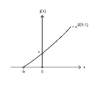
where [math]\displaystyle{ j(x) }[/math] is the "scaling" function and [math]\displaystyle{ \beta }[/math] and [math]\displaystyle{ \delta }[/math] are two critical-point exponents [3-7]. Thus, from (2) and (7), as the critical point is approached [math]\displaystyle{ (H\rightarrow 0 }[/math] and [math]\displaystyle{ t\rightarrow 0)\ , }[/math] [math]\displaystyle{ \mid H\mid }[/math] becomes a homogeneous function of [math]\displaystyle{ t }[/math] and [math]\displaystyle{ \mid M\mid ^{1/\beta} }[/math] of degree [math]\displaystyle{ \beta \delta\ . }[/math] The scaling function [math]\displaystyle{ j(x) }[/math] vanishes proportionally to [math]\displaystyle{ x+b }[/math] as [math]\displaystyle{ x }[/math] approaches [math]\displaystyle{ -b\ , }[/math] with [math]\displaystyle{ b }[/math] a positive constant; it diverges proportionally to [math]\displaystyle{ x^{\beta(\delta-1)} }[/math] as [math]\displaystyle{ x\rightarrow \infty\ ; }[/math] and [math]\displaystyle{ j(0) = c\ , }[/math] another positive constant (Fig. 1). Although (7) is confined to the immediate neighborhood of the critical point [math]\displaystyle{ (t, M, H }[/math] all near 0), the scaling variable [math]\displaystyle{ x = t/\mid M\mid ^{1/\beta} }[/math] nevertheless traverses the infinite range [math]\displaystyle{ -b \lt x \lt \infty\ . }[/math]

其中[math]\displaystyle{ j(x) }[/math]是“标度”函数，[math]\displaystyle{ \beta }[/math]和[math]\displaystyle{ \delta }[/math]是临界点指数。因此由(2)和(7)，当铁磁物质趋近于临界点时[math]\displaystyle{ (H\rightarrow 0 }[/math]且[math]\displaystyle{ t\rightarrow 0)\ , }[/math]，[math]\displaystyle{ \mid H\mid }[/math]是 [math]\displaystyle{ t }[/math] 和[math]\displaystyle{ \mid M\mid ^{1/\beta} }[/math]的[math]\displaystyle{ \beta \delta\ }[/math]次齐次函数。当[math]\displaystyle{ x }[/math]趋近于[math]\displaystyle{ -b\ }[/math]（正常数）时，标度函数[math]\displaystyle{ j(x) }[/math]趋近于零；当[math]\displaystyle{ x\rightarrow \infty\ ; }[/math]时，它发散至[math]\displaystyle{ x^{\beta(\delta-1)} }[/math]，且[math]\displaystyle{ j(0) = c\ }[/math]（正常数）（如图一）。尽管(7)局限在临界点[math]\displaystyle{ (t, M, H }[/math]都接近零）附近的极小范围内，但标度变量[math]\displaystyle{ x = t/\mid M\mid ^{1/\beta} }[/math]却遍历[math]\displaystyle{ -b \lt x \lt \infty\ }[/math]的无穷范围。

Scaling function [math]\displaystyle{ j(x) }[/math]

When [math]\displaystyle{ \mid H\mid = 0+ }[/math] and [math]\displaystyle{ t\lt 0\ , }[/math] so that [math]\displaystyle{ M }[/math] is then the spontaneous magnetization, we have from (7), [math]\displaystyle{ \mid M\mid = (-\frac{t}{b})^\beta\ , }[/math] where [math]\displaystyle{ \beta }[/math] is the conventional symbol for this critical-point exponent. When [math]\displaystyle{ M\rightarrow 0 }[/math] on the critical isotherm [math]\displaystyle{ (t=0)\ , }[/math] we have [math]\displaystyle{ H \sim cM\mid M\mid ^{\delta-1}\ , }[/math] where [math]\displaystyle{ \delta }[/math] is the conventional symbol for this exponent. From the first of the two properties of [math]\displaystyle{ j(x) }[/math] noted above, and Eq.(7), one may calculate the magnetic susceptibility [math]\displaystyle{ (\partial M/\partial H)_T\ , }[/math] which is then seen to diverge proportionally to [math]\displaystyle{ \mid t\mid ^{-\beta(\delta-1)}\ , }[/math] both at [math]\displaystyle{ \mid H\mid = 0+ }[/math] with [math]\displaystyle{ t\lt 0 }[/math] and at [math]\displaystyle{ H=0 }[/math] with [math]\displaystyle{ t\gt 0 }[/math] (although with different coefficients). The conventional symbol for the susceptibility exponent is [math]\displaystyle{ \gamma\ , }[/math] so we have [8]

[math]\displaystyle{ \label{eq:8} \gamma = \beta(\delta-1). }[/math]

Equations (7) and (8) are examples of scaling laws, Eq.(7) being a statement of homogeneity and the exponent relation (8) a consequence of that homogeneity.

当[math]\displaystyle{ \mid H\mid = 0+ }[/math]且[math]\displaystyle{ t\lt 0\ , }[/math][math]\displaystyle{ M }[/math]是自发磁化，从(7)可得[math]\displaystyle{ \mid M\mid = (-\frac{t}{b})^\beta\ , }[/math]其中[math]\displaystyle{ \beta }[/math]是这一临界指数的常用符号。在临界等温线[math]\displaystyle{ (t=0)\ , }[/math]当[math]\displaystyle{ M\rightarrow 0 }[/math]时，我们有[math]\displaystyle{ H \sim cM\mid M\mid ^{\delta-1}\ , }[/math]其中[math]\displaystyle{ \delta }[/math]是这一临界指数的常用符号。由前文中[math]\displaystyle{ j(x) }[/math]的第一个性质和式(7)，或可以计算磁化率[math]\displaystyle{ (\partial M/\partial H)_T\ , }[/math]，它在[math]\displaystyle{ \mid H\mid = 0+ }[/math]且[math]\displaystyle{ t\lt 0 }[/math]以及在[math]\displaystyle{ H=0 }[/math]且[math]\displaystyle{ t\gt 0 }[/math]时成比例发散至[math]\displaystyle{ \mid t\mid ^{-\beta(\delta-1)}\ }[/math]（尽管系数不同）。磁化率指数的常用符号是[math]\displaystyle{ \gamma\ , }[/math]因此有

[math]\displaystyle{ \gamma = \beta(\delta-1). }[/math]

(8)

方程(7)和(8)都是标度律的范例，(7)是齐次性的表述，(8)作为指数关系式则是这种齐次性的结果。

A free energy [math]\displaystyle{ F }[/math] may be obtained from (7) by integrating at fixed temperature, since [math]\displaystyle{ M = -(\partial F/\partial H)_T\ , }[/math] and the corresponding heat capacity [math]\displaystyle{ C_H }[/math] then follows from [math]\displaystyle{ C_H = -(\partial ^2 F/\partial T^2)_H\ . }[/math] One then finds from (7) that [math]\displaystyle{ C_H }[/math] at [math]\displaystyle{ H=0 }[/math] diverges at the critical point proportionally to [math]\displaystyle{ \mid t\mid ^{-\alpha} }[/math] (with different coefficients for [math]\displaystyle{ t\rightarrow 0- }[/math] and [math]\displaystyle{ t\rightarrow 0+)\ , }[/math] with the critical-point exponent [math]\displaystyle{ \alpha }[/math] related to [math]\displaystyle{ \beta }[/math] and [math]\displaystyle{ \gamma }[/math] by the scaling law [9]

[math]\displaystyle{ \label{eq:9} \alpha +2\beta +\gamma=2. }[/math]

由于[math]\displaystyle{ M = -(\partial F/\partial H)_T\ , }[/math]自由能[math]\displaystyle{ F }[/math]可以通过固定温度下积分由(7)式得出，且相应的热容[math]\displaystyle{ C_H = -(\partial ^2 F/\partial T^2)_H\ . }[/math]由(7)式可知，在[math]\displaystyle{ H=0 }[/math]时[math]\displaystyle{ C_H }[/math]在临界点处成比例发散至[math]\displaystyle{ \mid t\mid ^{-\alpha} }[/math]（其中[math]\displaystyle{ t\rightarrow 0- }[/math]和[math]\displaystyle{ t\rightarrow 0+)\ }[/math]各有不同的系数），临界点指数[math]\displaystyle{ \alpha }[/math]与[math]\displaystyle{ \beta }[/math]和[math]\displaystyle{ \gamma }[/math]满足以下标度律：

[math]\displaystyle{ \alpha +2\beta +\gamma=2. }[/math]

(9)

When [math]\displaystyle{ 2\beta+\gamma=2 }[/math] the resulting [math]\displaystyle{ \alpha =0 }[/math] means, generally, a logarithmic rather than power-law divergence together with a superimposed finite discontinuity occurring between [math]\displaystyle{ t=0+ }[/math] and [math]\displaystyle{ t=0- }[/math] [4]. In the 2-dimensional Ising model the discontinuity is absent and only the logarithm remains, while in mean-field (van der Waals, Curie-Weiss, Bragg-Williams) approximation the logarithm is absent but the discontinuity is still present.

当[math]\displaystyle{ 2\beta+\gamma=2 }[/math]，则有[math]\displaystyle{ \alpha =0 }[/math]，这通常意味着对数发散而不是幂律发散，并且在[math]\displaystyle{ t=0+ }[/math]和[math]\displaystyle{ t=0- }[/math]之间存在叠加有限不连续。在二维伊辛模型中，仅有对数关系而这种不连续是不存在的；而在平均场近似中情形相反。

Critical exponents 临界指数

What were probably the historically earliest versions of critical-point exponent relations like (8) and (9) are due to Rice [10] and to Scott [11]. It was before Domb and Sykes [12] and Fisher [13] had noted that the exponent [math]\displaystyle{ \gamma }[/math] was in reality greater than its mean-field value [math]\displaystyle{ \gamma =1 }[/math] but when it was already clear from Guggenheim's corresponding-states analysis [14] that [math]\displaystyle{ \beta }[/math] had a value much closer to 1/3 than to its mean-field value of 1/2. Then, under the assumption [math]\displaystyle{ \gamma =1 }[/math] and [math]\displaystyle{ \beta \simeq 1/3\ , }[/math] Rice had concluded from the equivalent of (8) that [math]\displaystyle{ \delta = 1+1/\beta \simeq 4 }[/math] (the correct value is now known to be closer to 5) and Scott had concluded from the equivalent of (9) that [math]\displaystyle{ \alpha =1-2\beta \simeq 1/3 }[/math] (the correct value is now known to be closer to 1/10). The mean-field values are [math]\displaystyle{ \delta =3 }[/math] and (as noted above) [math]\displaystyle{ \alpha =0\ . }[/math]

(8)和(9)分别来自里斯和斯考特的贡献。它们大概是历史上最早版本的临界指数关系。在此之后，Domb和Sykes以及Fisher注意到指数[math]\displaystyle{ \gamma }[/math]实际上比平均场值[math]\displaystyle{ \gamma =1 }[/math]大。而在更早之前，Guggenheim的对应状态分析就清楚地表明[math]\displaystyle{ \beta }[/math]值更靠近1/3而非平均场值的1/2.

The long-range spatial correlation functions in ferromagnets and fluids also exhibit a homogeneity of form near the critical point. At magnetic field [math]\displaystyle{ H=0 }[/math] (assumed for simplicity) the correlation function [math]\displaystyle{ h(r,t) }[/math] as a function of the spatial separation [math]\displaystyle{ r }[/math] (assumed very large) and temperature near the critical point (t assumed very small), is of the form [5,15]

[math]\displaystyle{ \label{eq:10} h(r,t)=r^{-(d-2+\eta)}G(r/\xi). }[/math]

[math]\displaystyle{ h(r,t)=r^{-(d-2+\eta)}G(r/\xi). }[/math]

(10)

Here [math]\displaystyle{ d }[/math] is the dimensionality of space, [math]\displaystyle{ \eta }[/math] is another critical-point exponent, and [math]\displaystyle{ \xi }[/math] is the correlation length (exponential decay length of the correlations), which diverges as

[math]\displaystyle{ \label{eq:11} \xi\sim \mid t\mid ^{-\nu} }[/math]

[math]\displaystyle{ \xi\sim \mid t\mid ^{-\nu} }[/math]

(11)

as the critical point is approached, with [math]\displaystyle{ \nu }[/math] still another critical-point exponent. Thus, [math]\displaystyle{ h(r,t) }[/math] (with [math]\displaystyle{ H=0) }[/math] is a homogeneous function of [math]\displaystyle{ r }[/math] and [math]\displaystyle{ \mid t\mid ^{-\nu} }[/math] of degree [math]\displaystyle{ -(d-2+\eta)\ . }[/math] The scaling function [math]\displaystyle{ G(x) }[/math] has the properties (to within constant factors of proportionality),

[math]\displaystyle{ \label{eq:12} G(x) \sim \left\{ \begin{array} {lc }x^{\frac{1}{2}(d-3)+\eta} e^{-x}, & x\rightarrow \infty \\ 1, & x\rightarrow 0 . \end{array} \right. }[/math]

[math]\displaystyle{ G(x) \sim \left\{ \begin{array} {lc }x^{\frac{1}{2}(d-3)+\eta} e^{-x}, & x\rightarrow \infty \\ 1, & x\rightarrow 0 . \end{array} \right. }[/math]

(12)

Thus, as [math]\displaystyle{ r\rightarrow \infty }[/math] in any fixed thermodynamic state (fixed t) near the critical point, [math]\displaystyle{ h }[/math] decays with increasing [math]\displaystyle{ r }[/math] proportionally to [math]\displaystyle{ r^{-\frac{1}{2}(d-1)}e^{-r/\xi}\ , }[/math] as in the Ornstein-Zernike theory. If, instead, the critical point is approached [math]\displaystyle{ (\xi \rightarrow \infty) }[/math] with a fixed, large [math]\displaystyle{ r\ , }[/math] we have [math]\displaystyle{ h(r) }[/math] decaying with [math]\displaystyle{ r }[/math] only as an inverse power, [math]\displaystyle{ r^{-(d-2+\eta)}\ , }[/math] which corrects the [math]\displaystyle{ r^{-(d-2)} }[/math] that appears in the Ornstein-Zernike theory in that limit. The scaling law(10) with scaling function [math]\displaystyle{ G(x) }[/math] interpolates between these extremes.

In the language of fluids, with [math]\displaystyle{ \rho }[/math] the number density and [math]\displaystyle{ \chi }[/math] the isothermal compressibility, we have as an exact relation in the Ornstein-Zernike theory

[math]\displaystyle{ \label{eq:13} \rho kT \chi =1+\rho \int h(r) \rm{d}\tau }[/math]

[math]\displaystyle{ \rho kT \chi =1+\rho \int h(r) \rm{d}\tau }[/math]

(13)

with [math]\displaystyle{ k }[/math] Boltzmann's constant and where the integral is over all space with [math]\displaystyle{ \rm{d} \tau }[/math] the element of volume. The same relation holds in the ferromagnets with [math]\displaystyle{ \chi }[/math] then the magnetic susceptibility and with the deviation of [math]\displaystyle{ \rho }[/math] from the critical density [math]\displaystyle{ \rho_c }[/math] then the magnetization [math]\displaystyle{ M\ . }[/math] At the critical point [math]\displaystyle{ \chi }[/math] is infinite and correspondingly the integral diverges because the decay length [math]\displaystyle{ \xi }[/math] is then also infinite. The density [math]\displaystyle{ \rho }[/math] is there just the finite positive constant [math]\displaystyle{ \rho_c }[/math] and [math]\displaystyle{ T }[/math] the finite [math]\displaystyle{ T_c\ . }[/math] Then from the scaling law (10), because of the homogeneity of [math]\displaystyle{ h(r,t) }[/math] and because the main contribution to the diverging integral comes from large [math]\displaystyle{ r\ , }[/math] where (10) holds, it follows that [math]\displaystyle{ \chi }[/math] diverges proportionally to [math]\displaystyle{ \xi^{2-\eta} \int G(x)x^{d-1}\rm{d} }[/math][math]\displaystyle{ x\ . }[/math] But the integral is now finite because, by (12), [math]\displaystyle{ G(x) }[/math] vanishes exponentially rapidly as [math]\displaystyle{ x\rightarrow \infty\ . }[/math] Thus, from (11) and from the earlier [math]\displaystyle{ \chi \sim \mid t\mid^{-\gamma} }[/math] we have the scaling law [15]

[math]\displaystyle{ \label{eq:14} (2-\eta)\nu = \gamma . }[/math]

[math]\displaystyle{ (2-\eta)\nu = \gamma . }[/math]

(14)

The surface tension [math]\displaystyle{ \sigma }[/math] in liquid-vapor equilibrium, or the analogous excess free energy per unit area of the interface between coexisting, oppositely magnetized domains, vanishes at the critical point (Curie point) proportionally to [math]\displaystyle{ (-t)^\mu }[/math] with [math]\displaystyle{ \mu }[/math] another critical-point exponent. The interfacial region has a thickness of the order of the correlation

length [math]\displaystyle{ \xi }[/math] so [math]\displaystyle{ \sigma/\xi }[/math] is the free energy per unit volume associated with the interfacial region. That is in its magnitude and in its singular critical-point behavior the same free energy per unit volume as in the bulk phases, from which the heat capacity follows by two differentiations with respect to the temperature. Thus, [math]\displaystyle{ \sigma/\xi }[/math] vanishes proportionally to [math]\displaystyle{ (-t)^{2-\alpha}\ ; }[/math] so, together with (9),

[math]\displaystyle{ \label{eq:15} \mu + \nu = 2-\alpha= \gamma +2\beta, }[/math]

[math]\displaystyle{ \mu + \nu = 2-\alpha= \gamma +2\beta, }[/math]

(15)

another scaling relation [16,17].

Exponents and space dimension

The critical-point exponents depend on the dimensionality [math]\displaystyle{ d\ . }[/math] The theory was found to be illuminated by treating [math]\displaystyle{ d }[/math] as continuously variable and of any magnitude. There is a class of critical-point exponent relations, often referred to as hyperscaling, in which [math]\displaystyle{ d }[/math] appears explicitly. The correlation length [math]\displaystyle{ \xi }[/math] is the coherence length of density or magnetization fluctuations. What determines its magnitude is that the excess free energy associated with the spontaneous fluctuations in the volume [math]\displaystyle{ \xi ^d }[/math] must be of order [math]\displaystyle{ kT\ , }[/math] which has the finite value [math]\displaystyle{ kT_c }[/math] at the critical point. But the typical fluctuations that occur in such an elemental volume are just such as to produce the conjugate phase. The free energy [math]\displaystyle{ kT }[/math] is then that for creating an interface of area [math]\displaystyle{ \xi^{d-1}\ , }[/math] which is [math]\displaystyle{ \sigma \xi^{d-1}\ . }[/math] Thus, as the critical point is approached [math]\displaystyle{ \sigma \xi^{d-1} }[/math] has a finite limit of order [math]\displaystyle{ kT_c\ . }[/math] Then from the definitions of the exponents [math]\displaystyle{ \mu }[/math] and [math]\displaystyle{ \nu\ , }[/math]

[math]\displaystyle{ \label{eq:16} \mu = (d-1)\nu, }[/math]

[math]\displaystyle{ \mu = (d-1)\nu, }[/math]

(16)

a hyperscaling relation [16]. With (15) we then have also [16]

[math]\displaystyle{ \label{eq:17} d\nu = 2-\alpha = \gamma+2\beta, }[/math]

[math]\displaystyle{ d\nu = 2-\alpha = \gamma+2\beta, }[/math]

(17)

which, with (8) and (14), yields also [18]

[math]\displaystyle{ \label{eq:18} 2-\eta = \frac{\delta -1}{\delta +1} d. }[/math]

[math]\displaystyle{ 2-\eta = \frac{\delta -1}{\delta +1} d. }[/math]

(18)

Unlike the scaling laws (8), (9), (14), and (15), which make no explicit reference to the dimensionality, the [math]\displaystyle{ d }[/math]-dependent exponent relations (16)-(18) hold only for [math]\displaystyle{ d\lt 4\ . }[/math] At [math]\displaystyle{ d=4 }[/math] the exponents assume the values they have in the mean-field theories but logarithmic factors are then appended to the simple power laws. Then for [math]\displaystyle{ d\gt 4\ , }[/math] the terms in the thermodynamic functions and correlation-function parameters that have as their exponents those given by the mean-field theories are the leading terms. The terms with the original [math]\displaystyle{ d }[/math]-dependent exponents, which for [math]\displaystyle{ d\lt 4 }[/math] were the leading terms, have been overtaken, and, while still present, are now sub-dominant.

This progression in critical-point properties from [math]\displaystyle{ d\lt 4 }[/math] to [math]\displaystyle{ d=4 }[/math] to [math]\displaystyle{ d\gt 4 }[/math] is seen clearly in the phase transition that occurs in the analytically soluble model of the ideal Bose gas. There is no phase transition or critical point in it for [math]\displaystyle{ d \le 2\ . }[/math] When [math]\displaystyle{ d\gt 2 }[/math] the chemical potential [math]\displaystyle{ \mu }[/math] (not to be confused with the surface-tension exponent [math]\displaystyle{ \mu }[/math]) vanishes identically for all [math]\displaystyle{ \rho \Lambda ^d \ge \zeta (d/2)\ , }[/math] where [math]\displaystyle{ \rho }[/math] is the density, [math]\displaystyle{ \Lambda }[/math] is the thermal de Broglie wavelength [math]\displaystyle{ h/\sqrt {2\pi mkT} }[/math] with [math]\displaystyle{ h }[/math] Planck's constant and [math]\displaystyle{ m }[/math] the mass of the atom, and [math]\displaystyle{ \zeta (s) }[/math] is the Riemann zeta function. As [math]\displaystyle{ \rho \Lambda^d \rightarrow \zeta(d/2) }[/math] from below, [math]\displaystyle{ \mu }[/math] vanishes through a range of negative values. As [math]\displaystyle{ \mu \rightarrow 0-\ , }[/math] the difference [math]\displaystyle{ \zeta(d/2)-\rho \Lambda^d }[/math] vanishes (to within positive proportionality factors) as

[math]\displaystyle{ \label{eq:19} \zeta(d/2)-\rho \Lambda^d \sim \left\{ \begin{array} {lc }(-\mu)^{d/2-1}, & 2\lt d\lt 4 \\ \\ \mu \ln(-\mu/kT), & d=4 \\ \\ -\mu , & d\gt 4 . \end{array}\right. }[/math]

[math]\displaystyle{ \zeta(d/2)-\rho \Lambda^d \sim \left\{ \begin{array} {lc }(-\mu)^{d/2-1}, & 2\lt d\lt 4 \\ \\ \mu \ln(-\mu/kT), & d=4 \\ \\ -\mu , & d\gt 4 . \end{array}\right. }[/math]

(19)

When [math]\displaystyle{ 2\lt d\lt 4 }[/math] the mean-field [math]\displaystyle{ -\mu }[/math] is still present but is dominated by [math]\displaystyle{ (-\mu)^{d/2-1}\ ; }[/math] when [math]\displaystyle{ d\gt 4 }[/math] the singular [math]\displaystyle{ (-\mu)^{d/2-1} }[/math] is still present but is dominated by the mean-field [math]\displaystyle{ -\mu\ . }[/math]

This behavior is reflected again in the Renormalization-group theory [19-21]. In the simplest cases there are two competing fixed points for the renormalization-group flows, one of them associated with [math]\displaystyle{ d }[/math]-dependent exponents that satisfy both the [math]\displaystyle{ d }[/math]-independent scaling relations and the hyperscaling relations, the other with the [math]\displaystyle{ d }[/math]-independent exponents of the mean-field theories [21]. The first determines the leading critical-point behavior when [math]\displaystyle{ d\lt 4\ . }[/math] At [math]\displaystyle{ d=4 }[/math] the two fixed points coincide and the exponents are now those of the mean-field theories but with logarithmic factors appended to the mean-field power laws. For [math]\displaystyle{ d\gt 4 }[/math] the two fixed points separate again and the leading critical-point behavior now comes from the one whose exponents are those of the mean-field theories. The effects of both fixed points are present at all [math]\displaystyle{ d\ , }[/math] but the dominant critical-point behavior comes from only the one or the other, depending on [math]\displaystyle{ d\ . }[/math]

Origin of homogeneity; block spins

A physical explanation for the homogeneity in (7) and (10) and for the exponent relations that are consequences of them is provided by the Kadanoff block-spin picture [5], which was itself one of the inspirations for the renormalization-group theory [19,20].

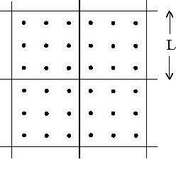
In a lattice spin model (Ising model), one considers blocks of spins, each of linear size [math]\displaystyle{ L\ , }[/math] thus containing [math]\displaystyle{ L^d }[/math] spins, with [math]\displaystyle{ L }[/math] much less than the diverging correlation length [math]\displaystyle{ \xi }[/math] (Fig. 2).

Block spins

Each block interacts with its neighbors through their common boundary as though it were a single spin in a re-scaled model. Each block is of finite size so the spins in its interior contribute only analytic terms to the free energy of the system. The part of the free-energy density (free energy per spin) that carries the critical-point singularities and their exponents comes from the interactions between blocks. Let this free-energy density be [math]\displaystyle{ f(t,H)\ , }[/math] a function of temperature through [math]\displaystyle{ t=T/T_c-1 }[/math] and of the magnetic field [math]\displaystyle{ H\ . }[/math] The correlation length is the same in the re-scaled picture as in the original, but measured as a number of lattice spacings it is smaller in the former by the factor [math]\displaystyle{ L\ . }[/math] Thus, the re-scaled model is effectively further from its critical point than the original was from its; so with [math]\displaystyle{ H }[/math] and [math]\displaystyle{ t }[/math] both going to 0 as the critical point is approached, the effective [math]\displaystyle{ H }[/math] and [math]\displaystyle{ t }[/math] in the re-scaled model are [math]\displaystyle{ L^xH }[/math] and [math]\displaystyle{ L^yt }[/math] with positive exponents [math]\displaystyle{ x }[/math] and [math]\displaystyle{ y\ , }[/math] so increasing with [math]\displaystyle{ L\ . }[/math] From the point of view of the original model the contribution to the singular part of the free energy made by the spins in each block is [math]\displaystyle{ L^df(t,H)\ , }[/math] while that same quantity, from the point of the view of the re-scaled model, is [math]\displaystyle{ f(L^yt, L^xH)\ . }[/math] Thus,

[math]\displaystyle{ \label{eq:20} f(L^yt, L^xH) \equiv L^df(t,H); }[/math]

[math]\displaystyle{ f(L^yt, L^xH) \equiv L^df(t,H); }[/math]

(20)

i.e., by (1), [math]\displaystyle{ f(t,H) }[/math] is a homogeneous function of [math]\displaystyle{ t }[/math] and [math]\displaystyle{ H^{y/x} }[/math] of degree [math]\displaystyle{ d/y\ . }[/math]

Therefore, by (2), [math]\displaystyle{ f(t,H)=t^{d/y} \phi(H^{y/x}/t)=H^{d/x}\psi(t/H^{y/x}) }[/math] where [math]\displaystyle{ \phi }[/math] and [math]\displaystyle{ \psi }[/math] are functions only of the ratio [math]\displaystyle{ H^{y/x}/t\ . }[/math] At [math]\displaystyle{ H=0 }[/math] the first of these gives [math]\displaystyle{ f(t,0)=\phi(0)t^{d/y}\ . }[/math] But two temperature derivatives of [math]\displaystyle{ f(t,0) }[/math] gives the contribution to the heat capacity per spin, diverging as [math]\displaystyle{ t^{-\alpha}\ ; }[/math] so [math]\displaystyle{ d/y=2-\alpha\ . }[/math] Also, on the critical isotherm [math]\displaystyle{ (t=0)\ , }[/math] the second relation above gives [math]\displaystyle{ f(0,H)=\psi(0)H^{d/x}\ . }[/math] But the magnetization per spin is [math]\displaystyle{ -(\partial f/\partial H)_T\ , }[/math] vanishing as [math]\displaystyle{ H^{d/x-1}\ , }[/math] so [math]\displaystyle{ d/x-1=1/\delta\ . }[/math] The exponents [math]\displaystyle{ d/x }[/math] and [math]\displaystyle{ d/y }[/math] have thus been identified in terms of the thermodynamic exponents: the heat-capacity exponent [math]\displaystyle{ \alpha }[/math] and the critical-isotherm exponent [math]\displaystyle{ \delta\ . }[/math] In the meantime, again with [math]\displaystyle{ -(\partial f/\partial H)_T }[/math] the magnetization per spin, the homogeneity of form of [math]\displaystyle{ f(t,H) }[/math] in (20) is equivalent to that of [math]\displaystyle{ H(t,M) }[/math] in (7), from which the scaling laws [math]\displaystyle{ \gamma=\beta(\delta-1) }[/math] and [math]\displaystyle{ \alpha + 2\beta + \gamma =2 }[/math] are known to follow.

A related argument yields the scaling law (10) for the correlation function [math]\displaystyle{ h(r,t)\ , }[/math] with [math]\displaystyle{ H=0 }[/math] again for simplicity. In the re-scaled model, [math]\displaystyle{ t }[/math] becomes [math]\displaystyle{ L^yt\ , }[/math] as before, while [math]\displaystyle{ r }[/math] becomes [math]\displaystyle{ r/L\ . }[/math] There may also be a factor, say [math]\displaystyle{ L^p }[/math] with some exponent [math]\displaystyle{ p\ , }[/math] relating the magnitudes of the original and rescaled functions; thus,

[math]\displaystyle{ \label{eq:21} h(r,t) \equiv L^{p}h(r/L,L^yt); }[/math]

[math]\displaystyle{ h(r,t) \equiv L^{p}h(r/L,L^yt); }[/math]

(21)

i.e., [math]\displaystyle{ h(r,t) }[/math] is homogeneous of degree [math]\displaystyle{ p }[/math] in [math]\displaystyle{ r }[/math] and [math]\displaystyle{ t^{-1/y}\ . }[/math] Then from the alternative form (2) of the property of homogeneity,

[math]\displaystyle{ \label{eq:22} h(r,t)\equiv r^p G(r/t^{-1/y}) }[/math]

[math]\displaystyle{ h(r,t)h(r,t)\equiv r^p G(r/t^{-1/y}) }[/math]

(22)

with a scaling function [math]\displaystyle{ G\ . }[/math] Comparing this with (10), and recalling that the correlation length [math]\displaystyle{ \xi }[/math] diverges at the critical point as [math]\displaystyle{ t^{-\nu} }[/math] with exponent [math]\displaystyle{ \nu\ , }[/math] we identify [math]\displaystyle{ p=-(d-2+\eta) }[/math] and [math]\displaystyle{ 1/y=\nu\ . }[/math] The scaling law [math]\displaystyle{ (2-\eta)\nu=\gamma\ , }[/math] which was a consequence of the homogeneity of form of [math]\displaystyle{ h(r,t)\ , }[/math] again holds, while from [math]\displaystyle{ 1/y=\nu }[/math] and the earlier [math]\displaystyle{ d/y=2-\alpha }[/math] we now have the hyperscaling law (17), [math]\displaystyle{ d\nu=2-\alpha\ . }[/math]

The block-spin picture thus yields the critical-point scaling of the thermodynamic and correlation functions, and both the [math]\displaystyle{ d }[/math]-independent and [math]\displaystyle{ d }[/math]-dependent relations among the scaling exponents. The essence of this picture is confirmed in the renormalization-group theory [19,20].

References

[1] C. Domb, The Critical Point (Taylor & Francis, 1996).

[2] M.E. Fisher, Repts. Prog. Phys. 30, part 2 (1967) 615.

[3] C. Domb and D.L. Hunter, Proc. Phys. Soc. 86 (1965) 1147.

[4] B. Widom, J. Chem. Phys. 43 (1965) 3898.

[5] L.P. Kadanoff, Physics 2 (1966) 263.

[6] A.Z. Patashinskii and V.L. Pokrovskii, Soviet Physics JETP 23 (1966) 292.

[7] R.B. Griffiths, Phys. Rev. 158 (1967) 176.

[8] B. Widom, J. Chem. Phys. 41 (1964) 1633.

[9] J.W. Essam and M.E. Fisher, J. Chem. Phys. 38 (1963) 802.

[10] O.K. Rice, J. Chem. Phys. 23 (1955) 169.

[11] R.L. Scott, J. Chem. Phys. 21 (1953) 209.

[12] C. Domb and M.F. Sykes, Proc. Roy. Soc. A 240 (1957) 214.

[13] M.E. Fisher, Physica 25 (1959) 521.

[14] E.A. Guggenheim, J. Chem. Phys. 13 (1945) 253.

[15] M.E. Fisher, J. Math. Phys. 5 (1964) 944.

[16] B. Widom, J. Chem. Phys. 43 (1965) 3892.

[17] P.G. Watson, J. Phys. C1 (1968) 268.

[18] G. Stell, Phys. Rev. Lett. 20 (1968) 533.

[19] K.G. Wilson, Phys. Rev. B 4 (1971) 3174.

[20] K.G. Wilson, Phys. Rev. B 4 (1971) 3184.

[21] K.G. Wilson and M.E. Fisher, Phys. Rev. Lett. 28 (1972) 240.

Internal references

• Tomasz Downarowicz (2007) Entropy. Scholarpedia, 2(11):3901.

• Eugene M. Izhikevich (2007) Equilibrium. Scholarpedia, 2(10):2014.

• Giovanni Gallavotti (2008) Fluctuations. Scholarpedia, 3(6):5893.

• Cesar A. Hidalgo R. and Albert-Laszlo Barabasi (2008) Scale-free networks. Scholarpedia, 3(1):1716.