曼德布洛特集

将不属于曼德布洛特集合内的点按照发散速度赋予不同的颜色所得到的图形/经过连续染色后曼德尔勃特集合(集合内染为黑色)

基于不同像素静态迭代数的曼德布洛特集动画

曼德布洛特集的细节部分

曼德布洛特集 Mandelbrot set 是对于复二次多项式 [math]\displaystyle{ f_c(z)=z^2+c }[/math]，在固定[math]\displaystyle{ z=0 }[/math]的前提下，所有使得无限迭代后的结果能保持有限数值（即不发散）的复数[math]\displaystyle{ c }[/math] 的集合。即满足数列 [math]\displaystyle{ f_c(0) }[/math], [math]\displaystyle{ f_c(f_c(0)) }[/math]等在绝对值中保持有界的复数[math]\displaystyle{ c }[/math]的集合。

放大后的曼德布洛特集

阿德里安 · 杜阿迪 Adrien Douady为纪念数学家伯努·瓦曼德布洛特 Benoît B. Mandelbrot将满足上述条件的集合命名为曼德布洛特集 。它与朱利亚集 Julia set有着很深的内在联系，朱利亚集也会产生与曼德布洛特集相类似的分形图案。

通过选取不同的复数[math]\displaystyle{ C }[/math]，观察其数列 [math]\displaystyle{ f_c(0), f_c(f_c(0)),\dotsc }[/math]是否达到无穷大（即其是否在预设的迭代次数后离开之前预设好的某个含0在内的有界领域）。将[math]\displaystyle{ C }[/math]的实部作为复平面图像 Complex Plane的横坐标，虚部作为复平面图像的纵坐标。 然后根据数列[math]\displaystyle{ |f_c(0)|,|f_c(f_c(0))|,\dotsc }[/math]。 若数列发散，则在二维平面内将所有属于集合内的点标记为黑色，不属于集合内的点按照发散速度赋予不同的颜色，就可以得到经典的曼德布洛特集图像。 需要注意的是，判断在无限迭代后其数列是否保持有界，是区分曼德布洛特集与其补集图像的有效方法。令复数C保持不变，取某一z值（如[math]\displaystyle{ z=z_0 }[/math]），可以得到数列[math]\displaystyle{ z_0,|f_c(z_0)|, |f_c(f_c(z_0))|,\dotsc }[/math]。这一数列可能发散于无穷大或始终处于某一范围之内并收敛于某一值。我们将使得该数列收敛于某值的z值的集合称为朱利亚集。若令[math]\displaystyle{ z_0 }[/math]取不同的值，则在简单函数的参数空间 Parameter Space中能够得到不同[math]\displaystyle{ z_0 }[/math]值所对应的朱利亚集。

 --木子二月鸟：曼德布洛特集图像可以通过选取不同的复数[math]\displaystyle{ C }[/math]，并观察其数列 [math]\displaystyle{ f_c(0), f_c(f_c(0)),\dotsc }[/math]是否达到无穷大（实践中通常指其是否在预设迭代次数后离开预设的某个含0在内的有界邻域）来实现：将[math]\displaystyle{ c }[/math]的实部作为复平面图像  Complex Plane的横坐标，虚部作为复平面图像的纵坐标，然后根据数列[math]\displaystyle{ |f_c(0)|,|f_c(f_c(0))|,\dotsc }[/math]超过主观设定阈值的速度来给每个点染色，若复数[math]\displaystyle{ C }[/math]的值在经过预设迭代次数之后没有超过阈值（注意：这里是将曼德布洛特集图像与其补集图像区分开来的标志）则染成特殊的颜色（通常是黑色）。如果复数[math]\displaystyle{ C }[/math]保持不变，而[math]\displaystyle{ z }[/math]的初始值——通常由[math]\displaystyle{ z_0 }[/math]来表示——却是一个变量，那么就能得到在简单函数的参数空间 Parameter Space中复数[math]\displaystyle{ C }[/math]对应的朱利亚集。

Images of the Mandelbrot set exhibit an elaborate and infinitely complicated boundary that reveals progressively ever-finer recursive detail at increasing magnifications. In other words, the boundary of the Mandelbrot set is a fractal curve. The "style" of this repeating detail depends on the region of the set being examined. The set's boundary also incorporates smaller versions of the main shape, so the fractal property of self-similarity applies to the entire set, and not just to its parts. The Mandelbrot set has become popular outside mathematics both for its aesthetic appeal and as an example of a complex structure arising from the application of simple rules. It is one of the best-known examples of mathematical visualization and mathematical beauty.

曼德布洛特集的图像展示了一条无比精致又无限复杂的分界线，将其不断的放大，就可看到更加精密的、基于递归的细节部分。也就是说，曼德布洛特集的分界线是一条分形曲线。重复出现的细部“样式”由所观测的集合区域所决定。曼德布洛特集的分界线上也包含了集合整体形状的较小版本，因此自相似性的分形特性不仅适用于该集合的局部，还适用于整个集合。 因为曼德布洛特集的图像在美学上拥有独特的吸引力，并且还是一个仅运用简单的运算规则就产生了复杂结构的代表例子。这使得曼德布洛特集在数学之外的其他领域中十分流行。它也是数学可视化和表现数学之美的最著名例子之一。

 --木子二月鸟：我觉得上面一段话的“分界线”还是用“边界”更为合适，因为曼德布洛特集的图形的边缘是一种分形的结果，而“分界线”容易让人以为内部的某些线条也是分形结果，可调整为：曼德布洛特集的图像展示了一条无比精致又无限复杂的边界线，将其不断的放大，就可看到更加精密的、基于递归的细节部分。也就是说，曼德布洛特集的边界线是一条分形曲线。重复出现的细部“样式”由经过计算（examined）的集合区域所决定。曼德布洛特集的边界线上也包含了集合整体形状的较小版本，因此自相似性的分形特性不仅适用于该集合的局部，还适用于整个集合。

因为曼德布洛特集的图像在美学上拥有独特的吸引力，并且还是一个根据简单规则产生复杂结构的代表例子，这使得曼德布洛特集在数学之外的其他领域中也十分流行。它也是数学可视化和表现数学之美的最著名例子之一。

历史

罗伯特·W·布鲁克斯和彼得·马特尔斯基在1978年发表了第一张曼德尔布洛特集的图像

The Mandelbrot set has its origin in complex dynamics, a field first investigated by the French mathematicians Pierre Fatou and Gaston Julia at the beginning of the 20th century. This fractal was first defined and drawn in 1978 by Robert W. Brooks and Peter Matelski as part of a study of Kleinian groups.[2] On 1 March 1980, at IBM's Thomas J. Watson Research Center in Yorktown Heights, New York, Benoit Mandelbrot first saw a visualization of the set.[3]Mandelbrot studied the parameter space of quadratic polynomials in an article that appeared in 1980.[4]

曼德尔洛特集起源于20世纪初由法国数学家皮埃尔费托 Pierre Fatou 和加斯顿茱莉亚 Gaston Julia 首先研究的复动力学。首次确切定义分形，并绘制出可视化的分形图案得益于 罗伯特·W·布鲁克斯 Robert W. Brooks和彼得·马特尔斯基 Peter Matelski在1978年对克莱尼群 Kleinian Groups 的部分研究工作。 在此基础上，1980年3月1日，在位于纽约的约克敦海茨 Yorktown Heights 的 IBM的 汤玛士·Ｊ·华生研究中心 Thomas J. Watson Research Center，伯努·瓦曼德布洛特 Benoît B. Mandelbrot首次绘制出曼德布洛特集的可视化图形。且Benoît B. Mandelbrot在1980年发表了一篇关于二次多项式 Quadratic Polynomials的参数空间 Parameter Space的研究论文。

 --趣木木（讨论） 2020年4月6日 (一) 04:12 (UTC)这里舍去 原文的人名  以之前在集智公众号上刊登的人名为主  查询后  本华·曼德博   法语： Benoît B. Mandelbrot，1924年11月20日－2010年10月14日 [1] ）又译伯努·瓦·曼德布洛特（该译名要规范一些）且与集合名称也更贴切一些 	
 --木子二月鸟：人名翻译没有问题，就是 complex dynamics 在百度百科和中国知网里中文文献里多是“复杂动力学”，待商榷。

对曼德布洛特集的数学研究真正始于数学家阿德里安· 杜阿迪 Adrien Douady 和约翰·H·哈伯德 John H. Hubbard 的一系列研究工作。他们探明了曼德布洛特集的许多基本性质，Adrien Douady 为纪念Benoît B. Mandelbrot在分形几何中做出的杰出贡献，将该集合命名为曼德布洛特集。

The mathematicians Heinz-Otto Peitgen and Peter Richter became well known for promoting the set with photographs, books,[5] and an internationally touring exhibit of the German Goethe-Institut.[6][7] The cover article of the August 1985 Scientific American introduced a wide audience to the algorithm for computing the Mandelbrot set. The cover featured an image located at -0.909 + -0.275 and was created by Peitgen, et al.[8][9] The Mandelbrot set became prominent in the mid-1980s as a computer graphics demo, when personal computers became powerful enough to plot and display the set in high resolution.[10]

数学家海因茨-奥托·佩特根 Heinz-Otto Peitgen 和彼得·里希特 Peter Richter 通过照片、书籍，在德国歌德学院 Goethe-Institut举办国际巡回展览等宣传方式，让曼德布洛特集进入大众的视野中，受到广泛的关注。 1985年8月《科学美国人 Scientific American 》的封面文章向广大读者介绍了计算曼德布洛特集的算法。20世纪80年代中期，当个人计算机的功能变得足够强大，可以绘制图形并以高分辨率显示这些图形时，曼德布洛特集被运用到计算机图形学的图像演示中，并日益凸显了它的重要性。

 --木子二月鸟： The cover featured an image located at -0.909 + -0.275 and was created by Peitgen, et al.没有翻译，可以考虑译为：该封面展示了一幅以(-0.909,-0.275)为坐标的曼德布洛特集图形，该图形由Peitgen创作。

The work of Douady and Hubbard coincided with a huge increase in interest in complex dynamics and abstract mathematics, and the study of the Mandelbrot set has been a centerpiece of this field ever since. An exhaustive list of all who have contributed to the understanding of this set since then is long but would include Mikhail Lyubich, Curt McMullen, John Milnor, Mitsuhiro Shishikura and Jean-Christophe Yoccoz. Curt McMullen, John Milnor, Mitsuhiro Shishikura and Jean-Christophe Yoccoz.

Adrien Douady和 John H. Hubbard 的研究工作不断取得新的成果，感兴趣于复动力学和抽象数学 Abstract Mathematics领域的队伍快速壮大，自此，深入了解曼德布洛特集一直是这些领域的核心研究。包括米哈伊尔 · 柳比奇 Mikhail Lyubich,[11][12] 科特 · 麦克马伦 Curt McMullen, 约翰 · 米尔诺 John Milnor, 石仓光博 Mitsuhiro Shishikura and 让-克里斯托夫·约科兹Jean-Christophe Yoccoz在内的许多人在曼德布洛特集的研究工作中，都作出了大大小小的贡献。

 --趣木木（讨论） 2020年4月6日 (一) 04:12 (UTC)第一句中的coincided weith 相吻合 换了并列句进行叙述
 --木子二月鸟： coincided with 应该是指两人的工作与人们对复杂动力学和抽象数学巨增的兴趣相吻合吧，建议改成：Adrien Douady和  John H. Hubbard 的工作与人们对复杂动力学和抽象数学兴趣的巨大增长相吻合，从那时起，对曼德布洛特集合的研究一直是这个领域的核心。尽管穷尽对理解曼德布洛特集有贡献的人名会非常长，但至少应包括米哈伊尔 · 柳比奇  Mikhail Lyubich,[11][12] 科特 · 麦克马伦   Curt McMullen, 约翰 · 米尔诺  John Milnor, 石仓光博 Mitsuhiro Shishikura 和 让-克里斯托夫·约科兹Jean-Christophe Yoccoz。

定义

The Mandelbrot set is the set of values of c in the complex plane for which the orbit of 0 under iteration of the quadratic map{\displaystyle z_{n+1}=z_{n}^{2}+c}remains bounded.[13]

曼德布洛特集是令复二次多项式 z_{n+1}=z_{n}^{2}+c中的Zn=0，将方程进行无限迭代，使其函数值构成的数列不发散的复数 c 的集合。[13]

 --木子二月鸟：曼德布洛特集是满足使得复二次多项式  z_{n+1}=z_{n}^{2}+c 自0开始进行迭代【从下句翻译得到的启发】并保持在有界范围内的复平面上的 c 的集合。

因此，该复数c满足以下条件：如果从 z0=0开始，进行重复迭代，所取的复数c使得zn 的绝对值都保持有界（不发散）。（对任意n>0） 例如，令 c=1，函数值数列为0,1,2,5,26，... ，发散，所以复数1∉曼德布洛特集。 令 c=-1，函数值数列是0,-1,0,-1,0，... ，收敛，所以复数-1∈曼德布洛特集。

一位数学家对曼德布洛特集进行了以下描述: 曼德布洛特集仅代表图中的黑色区域，即属于曼德布洛特集的复数c在黑色区域中，不属于曼德布洛特集的复数c在周围的白色区域中。 Re [ c ]和 Im [ c ]分别表示复数 c 的实部和虚部。

曼德布洛特集也可以定义为一族多项式 Polynomials的连通轨迹 Connectedness Locus。

基本性质

The Mandelbrot set is a compact set, since it is closed and contained in the closed disk of radius 2 around the origin. More specifically, a point {\displaystyle c}{ displaystyle c } belongs to the Mandelbrot set if and only if[math]\displaystyle{ |P_c^n(0)|\leq 2 }[/math] for all {\displaystyle n\geq 0.}

由于曼德布洛特集是一个封闭图形，且包含在以原点为中心，以2为半径的封闭圆盘中。故曼德布洛特集是一个紧集 Compact Set，更具体地说，若复数[math]\displaystyle{ c }[/math]属于曼德布洛特集，当且仅当对于 [math]\displaystyle{ n\geq 0. }[/math] 而言，其满足[math]\displaystyle{ |P_c^n(0)|\leq 2 }[/math] 。

 --木子二月鸟 后半句需要调整一下：更具体地说，对于 [math]\displaystyle{ n\geq 0. }[/math] 而言，当且仅当[math]\displaystyle{ |P_c^n(0)|\leq 2 }[/math]时，复数[math]\displaystyle{ c }[/math]属于曼德布洛特集。

In other words, if the absolute value of {\displaystyle P_{c}^{n}(0)} ever becomes larger than 2, the sequence will escape to infinity. 也就是说，若[math]\displaystyle{ |P_c^n(0)| }[/math]大于2，则说明其函数值数列发散，所对应的复数[math]\displaystyle{ c }[/math]不属于曼德布洛特集。

曼德布洛特集图像与逻辑斯蒂映射中的分叉图之间的关系

在y轴上对于Zn进行迭代，可以看到曼德布洛特集图像的收敛点处出现分叉

The intersection of {\displaystyle M} with the real axis is precisely the interval [−2, 1/4]. The parameters along this interval can be put in one-to-one correspondence with those of the real logistic family。

曼德布洛特集与复平面的实轴交点所构成的区间为[math]\displaystyle{ [−2, 1/4] }[/math]。属于该区间的参数c满足 逻辑斯蒂映射 Logistic Map的双射条件。 其中，逻辑斯蒂映射 Logistic Map是一种二次的多项式映射（递归关系式），是一个由简单非线性方程序产生混沌现象的经典范例。

 --趣木木（讨论） 2020年4月6日 (一) 04:12 (UTC)文中最后的logistic family链接与logistic map重定向，故统一译为Logistic Map。   其中，逻辑斯蒂映射 Logistic Map是一种二次的多项式映射（递归关系式），是一个由简单非线性方程序产生混沌现象的经典范例。 该句为补充
 --木子二月鸟 补充很赞！

[math]\displaystyle{ x_{n+1} = r x_n(1-x_n),\quad r\in[1,4]. }[/math]

其对应关系为 [math]\displaystyle{ z = r\left(\frac12 - x\right),\quad c = \frac{r}{2}\left(1-\frac{r}{2}\right). }[/math]

In fact, this gives a correspondence between the entire parameter space of the logistic family and that of the Mandelbrot set. 事实上，这反映了逻辑斯蒂映射和曼德布洛特集的参数空间 Parameter Space之间的对应关系。

关于曼德布洛特集是否连通，许多数学家都有过研究：

 --趣木木（讨论） 2020年4月6日 (一) 04:12 (UTC)所添加的过渡语句：“关于曼德布洛特集是否连通，许多数学家都有过研究：”

Douady and Hubbard have shown that the Mandelbrot set is connected. they constructed an explicit conformal isomorphism between the complement of the Mandelbrot set and the complement of the closed unit disk. Mandelbrot had originally conjectured that the Mandelbrot set is disconnected. This conjecture was based on computer pictures generated by programs that are unable to detect the thin filaments connecting different parts of {\displaystyle M} Upon further experiments, he revised his conjecture, deciding that {\displaystyle M} should be connected. There also exists a topological proof to the connectedness that was discovered in 2001 by Jeremy Kahn.[14]

Adrien Douady和 John H. Hubbard在曼德布洛特集的补集与闭合单位圆盘（以原点为中心，以1为半径做圆）的补集之间构造了一个显式的共形同构 Conformal Isomorphism ，由此证明了曼德布洛特集是连通的。 而由于当时计算机程序的局限性，导致程序无法检测到所生成的曼德布洛特集图形中连接不同细部的微小连线。Benoît B. Mandelbrot 最初猜测曼德布洛特集是不连通的。通过进一步的实验后，Benoît B. Mandelbrot 纠正了之前的看法，认为曼德布洛特集是连通的。 此外，杰里米 · 卡恩 Jeremy Kahn在2001年利用严格的拓扑证明，论证了曼德布洛特集的连通性。[14]

 --木子二月鸟 上面第二句的语序建议不要调整，因为在第一句叙述了“曼集是连通的。而由于当时计算机程序的局限性...”，这里的“当时”容易引起误解，以为是上句人物所处的时代，特别是该句最后还用了句号（如果用逗号可能会减少这种误解）。建议直译出来，也符合原文叙述的时间顺序：Benoît B. Mandelbrot 最初猜测曼德布洛特集是不连通的。这是由于当时计算机程序的局限性，导致程序无法检测到所生成的曼德布洛特集图形中连接不同细部的微小连线。

在曼德布洛特集运行一周期的附近的外部尾迹射线

The dynamical formula for the uniformisation of the complement of the Mandelbrot set, arising from Douady and Hubbard's proof of the connectedness of {\displaystyle M}，gives rise to external rays of the Mandelbrot set. These rays can be used to study the Mandelbrot set in combinatorial terms and form the backbone of the Yoccoz parapuzzle.[15]

由Adrien Douady和 John H. Hubbard证明曼德布洛特集连通时，所用到的曼德布洛特集的补集均匀化的动力学公式，引出了曼德布洛特集的外部尾迹射线。可将这些射线进行组合来研究曼德布洛特集，形成 Yoccoz parapuzzle 的骨架。 [15]

 --趣木木（讨论）	 form the backbone of the Yoccoz parapuzzle.[15]中的Yoccoz parapuzzle 暂不知道怎么翻译；点进链接为上文提出让-克里斯托夫·约科兹Jean-Christophe Yoccoz的页面 倾向于译为 形成了Jean-Christophe Yoccoz的对于该问题研究的理论框架
 --木子二月鸟 点进去看他的数学贡献，感觉可以将 Yoccoz parapuzzle  译为“Yoccoz 拼图/迷宫”？

The boundary of the Mandelbrot set is exactly the bifurcation locus of the quadratic family; that is, the set of parameters {\displaystyle c} for which the dynamics changes abruptly under small changes of {\displaystyle c.} It can be constructed as the limit set of a sequence of plane algebraic curves, the Mandelbrot curves, of the general type known as polynomial lemniscates. The Mandelbrot curves are defined by setting p0 = z, pn+1 = pn2 + z, and then interpreting the set of points |pn(z)| = 2 in the complex plane as a curve in the real Cartesian plane of degree 2n+1 in x and y. These algebraic curves appear in images of the Mandelbrot set computed using the "escape time algorithm" mentioned below.

曼德布洛特集的分界线是二次族 bifurcation locus的分岔轨迹，即参数c在极微小的变化下会产生很突然的波动情况。该分界线是一类多项式双曲线，可被构造成一系列平面代数曲线的极限集。 通过设置 p₀ = z, p_n+1 = p_n² + z，然后将复平面上的点集p_n(z)| = 2 转化为实笛卡尔平面 Cartesian Plane上度为ⁿ⁺¹的在 x 和 y 上的曲线，从而对该曲线进行定义。 使用下面所提及的“逃逸时间算法”计算并绘制出来的曼德布洛特集图像中也显示了该分界线。

 --木子二月鸟 曼德布洛特集的边界是二次族 quadratic family的分岔轨迹 bifurcation locus，即参数c在极微小的变化下会产生很突然的动力学变化。另外，度为2n+1

其他性质

心脏形结构和圆盘形“芽苞”Main cardioid and period bulbs

双曲分量的周期

Upon looking at a picture of the Mandelbrot set, one immediately notices the large cardioid-shaped region in the center. This main cardioid is the region of parameters {\displaystyle c} for which {\displaystyle P_{c}} has an attracting fixed point. It consists of all parameters of the form {\displaystyle c={\frac {\mu }{2}}\left(1-{\frac {\mu }{2}}\right)} for some {\displaystyle \mu } in the open unit disk. 观察曼德布洛特集的图像，会首先看到中间的心脏形结构。（即图11中的区域1）该心形曲线内部的参数[math]\displaystyle{ c }[/math]若满足[math]\displaystyle{ c = \frac\mu2\left(1-\frac\mu2\right) }[/math]， 其中 [math]\displaystyle{ \mu }[/math] 属于单位开圆盘； 则称这样的点[math]\displaystyle{ c }[/math]，为复二次映射的周期点，记作[math]\displaystyle{ P_c }[/math]。

 --木子二月鸟:这里有术语无能为力：open unit disk（开放单位圆盘？）

[图片12：To the left of the main cardioid, attached to it at the point {\displaystyle c=-3/4}, a circular-shaped bulb is visible. This bulb consists of those parameters {\displaystyle c} for which {\displaystyle P_{c}} has an attracting cycle of period 2. This set of parameters is an actual circle, namely that of radius 1/4 around −1. （图12）在主心形线的左侧，点（-3/4，0）处，能够看到一个圆盘形的“芽苞”突起。该“芽苞”由一周期2的吸性周期循环的参数c的集合组成，其为曼德布洛特集的一个附属子集。该子集组成了以（-1，0）为中心，以1/4 为半径的圆形区域。]

类似这样的“芽苞”突起有无穷多个，它们都与主心脏形结构曲线相切。 且满足以下定义： 对于任意有理数 [math]\displaystyle{ \tfrac{p}{q} }[/math] ，p、q互素，若参数c满足：

[math]\displaystyle{ c_{\frac{p}{q}} = \frac{e^{2\pi i\frac pq}}2\left(1-\frac{e^{2\pi i\frac pq}}2\right). }[/math]

则该点处存在一个与主心脏形结构曲线相切的"芽苞"，且记作“ [math]\displaystyle{ \tfrac{p}{q} }[/math]-芽苞”。

在 Julia 集上绘制一周期为2 / 5的吸性周期循环的“芽苞”(动画)

[math]\displaystyle{ c_{\frac{p}{q}} = \frac{e^{2\pi i\frac pq}}2\left(1-\frac{e^{2\pi i\frac pq}}2\right) }[/math]公式中的参数其由吸性循环周期的周期值q和组合旋转数 [math]\displaystyle{ \tfrac{p}{q} }[/math] 组成。包含周期为q的吸性周期循环的Factou 集 Fatou components 都在吸性不动点相交。若记分量[math]\displaystyle{ U_0,\dots,U_{q-1} }[/math]为逆时针方向，[math]\displaystyle{ P_c }[/math]将分量[math]\displaystyle{ U_j }[/math] 映射到分量[math]\displaystyle{ U_{j+p\,(\operatorname{mod} q)} }[/math]

吸性周期为 1/2, 3/7, 2/5, 1/3, 1/4, and 1/5 “芽苞”的朱利亚基

周期和分枝

The change of behavior occurring at {\displaystyle c_{\frac {p}{q}}} is known as a bifurcation: the attracting fixed point "collides" with a repelling period q-cycle. As we pass through the bifurcation parameter into the {\displaystyle {\tfrac {p}{q}}}-bulb, the attracting fixed point turns into a repelling fixed point (the {\displaystyle \alpha }-fixed point), and the period q-cycle becomes attracting. [math]\displaystyle{ c_{\frac{p}{q}} }[/math] 为分枝 Bifurcation点，在该点吸性的不动点与斥性的周期循环发生相反的变化。当经过分枝点进入[math]\displaystyle{ \tfrac{p}{q} }[/math]-“芽苞”时，即[math]\displaystyle{ c_{\frac{p}{q}} }[/math] 从心脏形结构曲线内部变为开圆内部时，不动点[math]\displaystyle{ \alpha }[/math]由吸性变为斥性，周期循环由斥性变为吸性。

趣木木（讨论） "collides" with 相冲突 译为发生相反的变化，即后文所说的“不动点由吸性变为斥性，周期循环由斥性变为吸性。”

双曲分量 Hyperbolic components

上述所提及的圆盘形“芽苞”都是曼德布洛特集的内部分量，其中映射[math]\displaystyle{ P_{c} }[/math]具有吸性周期循环，这样的分量称为双曲分量。

推测这些双曲分量是否仅存在于曼德布洛特集内部区域，称为双曲密度问题。这或许也是复动力学领域中最值得关注的公开问题。曼德布洛特集中假设的非双曲分量通被称为“怪胎”或幽灵分量。[16]

[17]对于实二次多项式，在1990年，双曲密度问题得到解决。柳比奇 Lyubich 、格拉奇克 Graczyk、斯维亚特克 Świątek分别独立证明了双曲分量仅存在于曼德布洛特集的内部区域。

Not every hyperbolic component can be reached by a sequence of direct bifurcations from the main cardioid of the Mandelbrot set. However, such a component can be reached by a sequence of direct bifurcations from the main cardioid of a little Mandelbrot copy (see below). 并不是每个双曲分量都可由曼德布洛特集的主心脏形结构经过一系列的直接分叉即可得到。但像图（15）的双曲分量可由小的曼德布洛特集副本的主心脏结构曲线经过一系列的直接分叉得到。

每个双曲分量都有一个中心，该中心记作点[math]\displaystyle{ c }[/math]，使得[math]\displaystyle{ P_{c}（z） }[/math]的内部Fatou区域具有一个超吸性周期循环，即其吸引力是无穷的。这意味着该循环包含临界点0，因此经过数次迭代后，0会回到本身。

We therefore have that {\displaystyle P_{c}}n{\displaystyle (0)=0} for some n. If we call this polynomial {\displaystyle Q^{n}(c)} (letting it depend on c instead of z), we have that {\displaystyle Q^{n+1}(c)=Q^{n}(c)^{2}+c} and that the degree of {\displaystyle Q^{n}(c)} is {\displaystyle 2^{n-1}}. We can therefore construct the centers of the hyperbolic components by successively solving the equations {\displaystyle Q^{n}(c)=0,n=1,2,3,...}. The number of new centers produced in each step is given by Sloane's OEIS: A00074 也就是说，将0带入[math]\displaystyle{ P_{c}（z） }[/math]，存在n,使得[math]\displaystyle{ P_c }[/math]ⁿ[math]\displaystyle{ (0) = 0 }[/math]。 如果将公式的变量固定为[math]\displaystyle{ c }[/math]而不是[math]\displaystyle{ z }[/math],得到 [math]\displaystyle{ Q^{n}(c) }[/math]。 由[math]\displaystyle{ Q^{n+1}(c) = Q^{n}(c)^{2} + c }[/math]，且令[math]\displaystyle{ Q^{n}(c)的纬度为2^{n-1} }[/math]。 因此，我们可以通过依次求解方程[math]\displaystyle{ Q^{n}(c) = 0, n = 1, 2, 3, ... }[/math]来构造双曲分量的中心。每一步产生的新中心的个数由斯隆的OEIS: A00074给出。OEIS的全称为：The On-Line Encyclopedia of Integer Sequences™ (OEIS™)，它是一个关于整数序列（数列）的专业型网站，是一个关于组合数学研究的重要的网站，里面包含了众多数列的研究成果。 趣木木（讨论）解释一下OEIS的一些简单内容“ OEIS的全称为：The On-Line Encyclopedia of Integer Sequences™ (OEIS™)，它是一个关于整数序列（数列）的专业型网站，是一个关于组合数学研究的重要的网站，里面包含了众多数列的研究成果。”

连通性 Local connectivity

没有曼德布洛特集的微小副本和 Misiurewicz 点的曼德布洛特拓扑模型(Cactus 模型)

曼德布洛特集的Thurston模型(摘要曼德布洛特集）

在Adrien Douady 和 John H. Hubbard的研究工作中，提出了著名的MLC猜想：他们推测曼德布洛特集是局部连通的。这一猜想将曼德布洛特集简单抽象成一个“压缩圆盘”。 其中，它还体现了上述所提及的双曲分量的思想。

让-克里斯托夫·约科兹 Jean-Christophe Yoccoz证明了在所有有限可重整化参数下的曼德布洛特集的局部连通性; 也就是说，该种局部连通性只体现在有限多个小曼德布洛特集副本中。 [18]从那时起，在曼德布洛特集的其他参数点也体现了局部连通性。

自相似 Self-similarity

曼德布洛特集中的自相似性通过放大一个圆形“芽苞”，并将其中心往负x轴方向迁移来体现。从(- 1,0)到(- 1.31,0) ，而视图从0.5x0.5放大到0.12x0.12，以接近 Feigenbaum 比率Ħẟ

在Misiurewicz点−0.1011 + 0.9563i附近的自相似性

在 Misiurewicz 点附近，对曼德布洛特集进行放大，能够观察到自相似性。将其收敛于一个极限集后，我们还推测在广义 Feigenbaum 点(例如-1.401155或-0.1528 + 1.0397 i)周围能够观察到自相似的特征。 [19][20]

曼德布洛特集中的准自相似性

总的来说，曼德布洛特集合并不是严格意义上的具有自相似特征的集合，但它具有准自相似性，因为在任意小的空间尺度上，都可以找到与自身略有不同的小副本。小副本之间的细微差别体现在它们与整体集合之间的连接细线上。

进一步的计算结果 Further results

Mitsuhiro Shishikura计算出曼德布洛特集分界线的豪斯多夫维数 Hausdorff dimension 为2。 现在还不知道曼德布洛特集分界线是否具有正平面上的勒贝格测度 Lebesgue Measure。

In the Blum-Shub-Smale model of real computation, the Mandelbrot set is not computable, but its complement is computably enumerable. However, many simple objects (e.g., the graph of exponentiation) are also not computable in the BSS model. At present, it is unknown whether the Mandelbrot set is computable in models of real computation based on computable analysis, which correspond more closely to the intuitive notion of "plotting the set by a computer". Hertling has shown that the Mandelbrot set is computable in this model if the hyperbolicity conjecture is true. 利用可在实数域内计算的 Blum-Shub-Smale 模型 Blum-Shub-Smale Model （简称BBS模型），可得出以下结论：虽然无法对于曼德布洛特集进行计算，但可计算其补集。BBS模型也不可计算包括求幂图在内的许多比较简单的图像。目前，在基于可计算性分析 Computable Analysis的实际计算模型中，曼德布洛特集是否可算尚未有定论。由该种模型计算集合的方式更接近于直观概念上的“由计算机绘制集合”。 赫特林 Hertling 证明了若双曲性猜想是正确的，则该模型中的曼德布洛特也是可计算的。

 --木子二月鸟 这句的翻译待商榷：At present, it is unknown whether the Mandelbrot set is computable in models of real computation based on computable analysis, which correspond more closely to the intuitive notion of "plotting the set by a computer". 一处是real computation 应为实数域，另一处是目前的译法“由该种模型计算集合的方式...”中“该种模型”指代不清。可以考虑调整为：

目前，在基于可计算性分析 Computable Analysis（该种分析方式更接近于直观概念上的“由计算机绘制集合”）的实数域模型中，曼德布洛特集是否可计算尚未有定论。

将曼德布洛特集进行放大，可观察到朱利亚岛和一个与朱利亚集很相似的结构

与朱利亚集之间的关系

朱利亚集 Julia set可由[math]\displaystyle{ f_c(z)=z^2+c }[/math]反复迭代得到。与曼德布洛特集不同，其对于复数[math]\displaystyle{ c }[/math]进行固定，取某一个[math]\displaystyle{ z }[/math]值，（如[math]\displaystyle{ z=z_0 }[/math]），可以得到数列[math]\displaystyle{ z_0,f_c(z_0),f_c(f_c(z_0)),f_c(f_c(f_c(z_0))).... }[/math]。该数列可能趋于无穷大或者始终处于某一范围之内并收敛于某一值。将使该数列不发散的[math]\displaystyle{ z }[/math]值集合称为朱利亚集。

由曼德布洛特集的定义，在给定点处曼德布洛特集的几何结构与相应的朱利亚集的几何结构有着密切的对应关系。 例如，当一个点在曼德布洛特集聚集时，相应的朱利亚集是连通的。

事实上，该原理被运用到曼德布洛特集的所有深层结果中。 例如，Shishikura 证明了对于在曼德布洛特集分界线上的一组稠密的参数，相对应的朱利亚集 Julia set的豪斯多夫维数为2，然后将这些信息传递到参数平面上。 [21]同样，Yoccoz 首先证明了朱利亚集的局部连通性，然后在相应的参数点处进一步证明曼德布洛特集的局部连通性。 [18]Adrien Douady将这一原则表述为:在动力平面上耕耘，在参数空间中收获。

几何结构

主心脏形结构上带有7-13个天线的8-14个周期图案

对于任意有理数[math]\displaystyle{ \tfrac{p}{q} }[/math]，其中p 和q互素，周期 q 的一个双曲分量从主心脏形结构分支出来。 在该分枝点上与主心脏形结构相连的曼德布洛特集部分称为 p / q-limb。 计算机实验表明，分枝体半径像[math]\displaystyle{ \tfrac{1}{q^2} }[/math]一样趋于0，目前最佳的拟合形式是约科兹不等式 Yoccoz-inequality，其尺寸像[math]\displaystyle{ \tfrac{1}{q} }[/math]一样趋于0。 周期为[math]\displaystyle{ q }[/math]的分枝体顶端有[math]\displaystyle{ q-1 }[/math]个天线。我们可以通过计数这些触角反过来推算该特定分枝体的周期为多少。

曼德布洛特集中的π

为了证明 p / q-limb 的厚度为零，大卫·鲍尔 David Boll 在1991年利用计算机计算了使得 [math]\displaystyle{ z =-\tfrac{3}{4} + i\epsilon }[/math] ([math]\displaystyle{ -\tfrac{3}{4} }[/math]的级数发散所需的迭代次数。（[math]\displaystyle{ -\tfrac{3}{4} }[/math]是所处的位置）。由于z = [math]\displaystyle{ -\tfrac{3}{4} }[/math]为确切值，并不发散。则需要进一步缩小 ε、增加迭代次数，更加接近目标值。譬如：当ε = 0.0000001时，需迭代31415928次，此时输出值的π值为3.1415928。[22]

曼德布洛特集中的斐波那契数列

可以看出，斐波那契数列 Fibonacci Sequence位于曼德布洛特集内，且与主心脏形结构曲线和法雷数列图存在关联。

将主心脏结构曲线映射到一个圆盘上时，会观察到由下一个最大的双曲分量延伸出来的天线，其位于之前选择的两个分量之间。天线的数目变化是一个斐波那契数列。

The amount of antennae also correlates with the Farey Diagram and the denominator amounts within the corresponding fractional values, of which relate to the distance around the disk. Both portions of these fractional values themselves can be summed together after {\frac {1}{3}}to produce the location of the next Hyperbolic component within the sequence. Thus, the Fibonacci sequence of 1, 2, 3, 5, 8, 13, and 21 can be found within the Mandelbrot set. 天线数目也与法雷数列图有关，由于n级法雷数列是指对任意给定的一个自然数n，将分母小于等于n的不可约的真分数按升序排列，并且在第一个分数之前加上0/1，在最后一个分数之后加上1/1所得到的数列，以[math]\displaystyle{ F_n }[/math]表示。如[math]\displaystyle{ F_5 }[/math]为：0/1, 1/5, 1/4, 1/3, 2/5, 1/2, 3/5, 2/3, 3/4, 4/5, 1/1。

可得到：在曼德布洛特集中的法雷数列，其分母数量在相应的分数值内，分数值与圆盘周围的距离有关。这两个部分的分数值本身可以在[math]\displaystyle{ {\frac{1}{3}} }[/math]之后相加，以计算出序列中下一个双曲分量的位置。因此，在曼德尔勃特集合中可以找到1、2、3、5、8、13和21的斐波那契数列。

 --趣木木（讨论）对于法雷数列进行解释“对任意给定的一个自然数n，将分母小于等于n的不可约的真分数按升序排列，并且在第一个分数之前加上0/1，在最后一个分数之后加上1/1，这个序列称为n级法雷数列，以Fn表示。###再看再思考

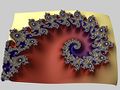
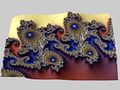
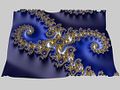
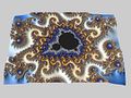
不同缩放比率下的图像库

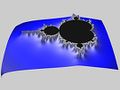
当一个人看得越近或放大图像时，达到的放大效果可以让曼德布洛特集显示出更复杂的细节。当将下图不断的放大，缩放到选定的[math]\displaystyle{ c }[/math]值形成一个反映其变化的图集时，会给人一种不同几何结构中蕴藏着无限想象力的感觉。下也对于它们的一些典型规则进行说明。

• 

  开始：将曼德布洛特集进行着色，以便于观察

• 

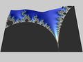
  主心脏形结构和第二大圆盘之间的空隙称为“海马谷”

• 

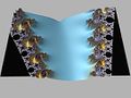
  左边是双螺旋，右边是“海马”

• 

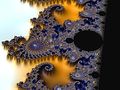
  颠倒过来的海马

The magnification of the last image relative to the first one is about 1010 to 1. Relating to an ordinary monitor, it represents a section of a Mandelbrot set with a diameter of 4 million kilometers. Its border would show an astronomical number of different fractal structures. 图27相对于图24的放大倍率之比约为1010：1。以普通的显示器显示出该图像的完整图形，其表示直径为400万公里的的曼德布洛特集合的一部分，其分界线将显示出数量庞大的不同分形结构。

 --趣木木（讨论）以显示器有关  觉得应该是指  按照图27的缩放倍率将整个图像进行填充  讨论最后成型的图形
 --木子二月鸟：这里第一句中的放大倍数应是10的10次方吧，粘贴到百科时格式没有了。它这里说的最后一幅图是指Image gallery of a zoom sequence里的最后第16幅图吧？

海马的“身体”由25个“辐条”组成。25个“辐条”被分为三组，其中两组中各含有12个“辐条”，另一组单独由一个连接到主心脏形结构的“辐条”组成。这各含有12个“辐条”的两组可以通过某种变形变集合的“上臂”为曼德布洛特集的两根“手指”；中心是通常说的 Misiurewicz 点。在海马的“身体的上半部分”和“尾巴”之间，可发现一个扭曲的曼德布洛特集的小副本。该集合称为“卫星集”，也就是附属集。

• 

  “海马尾巴”的中心端点也是 Misiurewicz 点。

• 

  海马“尾巴”的一部分ーー只有一条路径是由贯穿整个“尾巴”的细小结构组成的。 这条曲折的路径穿过大型物体的”中心” ，在”尾部”的内外边界上有25个”辐条” ; 因此曼德布洛特集是一个单连通集，这意味着在洞周围没有岛屿和环路。

• 

  卫星集。这两个“海马尾”是一系列同心冠的源头，冠的中心是卫星集。 在交互式查看器中打开此位置。

• 

  每个冠都由类似的“海马尾”组成; 它们的数量随着2的幂数增加而增加，这是卫星环境中的典型现象。通向螺旋中心的独特路径将卫星从心形的凹槽传递到“头”上的“天线”顶部

• 

  卫星的“天线”。可以辨认出几颗二级卫星。

• 

  卫星的“海马谷”。所有的结构以一开始的图形样式再次出现

• 

  双螺旋和“海马”——与第二张图片开始时不同，它们有附属结构，如“海马尾” ; 这展示了 n + 1个不同结构在 n 阶卫星环境中的典型连接，最简单的情况是 n = 1。

• 

  具有二级卫星的双螺旋——类似于“海马” ，双螺旋由“天线”演化而来

• 

  能够辨认出附属集的外部岛结构，它们的形状类似于朱利亚集[math]\displaystyle{ J_c }[/math].其中最大的岛结构可在右侧的“双钩”中心找到。

• 

  “双钩”的一部分

• 

  岛群

• 

  一个岛屿的细节部分

• 

  其中一个螺旋的细节部分，利用交互式查看器中打开

上面的岛屿似乎是由无限多的部分组成，就像康托集 Cantor Sets一样。但实际上这是对应的朱利亚集[math]\displaystyle{ J_c }[/math]的情况。然而，它们通过微小的结构进行连接，其整体代表了一个单连通集。

这些微小的结构在中间的卫星集处相遇，在这样的放大倍率下，该卫星集太小以至于无法被识别。相应的[math]\displaystyle{ J_c }[/math] 的[math]\displaystyle{ c }[/math]值不是该图像中心所对应的[math]\displaystyle{ c }[/math]值，而是第六个缩放步骤中，相对于曼德布洛特集的主体，其中心所示的相同位置上的卫星集所对应的[math]\displaystyle{ c }[/math]值。

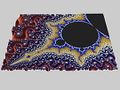
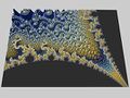
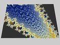
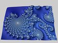
曼德布洛特集和朱利亚集的3D图像

除了能绘制出曼德布洛特集的二维图像外，还可以利用各种技术绘制出曼德布洛特集和朱利亚集的三维图像。具体做法为：将其二维图像中的每个像素赋予一个高度值，即可生成三维图像。

最简单的三维图像渲染方法是将每个像素的迭代值作为高度值，从而生成具有不同高度值的“台阶”的图像。

利用整数迭代渲染曼德布洛特集的三维图像

如果使用分数迭代值(也称为势函数[23])来计算每个点的高度值，则可以避免在生成的图像中执行步骤。 然而，使用分数迭代数据渲染的三维图像看起来比较粗糙且不太美观。

利用分数迭代渲染曼德布洛特集的三维图像

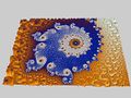
另一种方法是使用每个点的距离估计[24](DE)数据来计算高度值。利用指数函数对距离估计值进行非线性映射，可以得到感观较好的图像。使用 DE 数据绘制的图像往往在视觉上更引人关注。更重要的是，三维图像使得连接图像中各点的细“卷须”更易于观察。 在“分形图像的科学”第121页的图29、30显示了使用外部距离估计绘制的二维和三维图像。

利用距离估计渲染曼德布洛特集的三维图像。

Below is a 3D version of the "Image gallery of a zoom sequence" gallery above, rendered as height maps using Distance Estimate data, and using similar cropping and coloring. 下面是“一直缩放的三维曼德布洛特集图集”，在高度值图中利用距离估计将其进行渲染，并使用类似的裁剪和着色。

 --趣木木（讨论）height maps可以理解为高度值组成的图吗？
 --木子二月鸟：我觉得是这个意思，不过第一个短句是不是改为“以下是前面“不断缩放的曼德布洛特集图集”的3D版本”。

 --趣木木（讨论）下面的图形注释翻译与上文某处一致 只是对于不同的显示图形  渲染方式不同

• 

  zoom 00:开始，曼德布洛特集进行一系列的着色

• 

  zoom 01:“头部”和“身体”之间的空隙，也称为“海马谷”

• 

  zoom 02:左边是双螺旋，右边是“海马”

• 

  zoom 03:颠倒后的“海马”

• 

  zoom 04:海马尾

• 

  zoom 05:海马尾的一部分

• 

  zoom 06:拥有一对“海马尾”的卫星集

• 

  zoom 07:卫星集的特写

• 

  zoom 08:卫星的“天线”，可以识别出几颗二级卫星。

• 

  zoom 09:卫星的“海马谷”。所有的结构以一开始的图形样式再次出现

• 

  zoom 10:双螺旋和“海马”

• 

  zoom 11:二级卫星的双螺旋

• 

  Zoom 12.

• 

  Zoom 13:“双钩”的一部分

• 

  Zoom 14:岛群

• 

  Zoom 15:一个岛的细节部分

• 

  Zoom 16:螺旋的细节部分

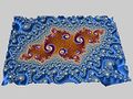
下图类似于上图中的“zoom 05”，它来自于《分形之美》这本书的第85页图44的3D图像版本。

《分形之美》这本书的第85页图44的曼德布洛特集的3D图像版本

推广 Generalizations

左从0到5，右从0.05到2的多重曼德布洛特集的动画。--薄荷(右侧视频无法加载)

由于四维曼德布洛特集可以通过投影或横切成三维，故四维朱利亚集也可以进行该种变换

多重曼德布洛特集 Multibrot sets

Multibrot sets are bounded sets found in the complex plane for members of the general monic univariate polynomial family of recursions {\displaystyle z\mapsto z^{d}+c.\ } 在数学中，Multibrot集是复平面上的有限集，集中的元素取自一般一元多项式递归族中。如： [math]\displaystyle{ z \mapsto z^d + c.\ }[/math] 这个名字是多重和曼德布洛特集的混合词。同样的也适用于朱利亚集合，称为多重朱利亚集 Multi-Julia set。

For an integer d, these sets are connectedness loci for the Julia sets built from the same formula. The full cubic connectedness locus has also been studied; here one considers the two-parameter recursion {\displaystyle z\mapsto z^{3}+3kz+c}, whose two critical points are the complex square roots of the parameter k. A parameter is in the cubic connectedness locus if both critical points are stable.[26] For general families of holomorphic functions, the boundary of the Mandelbrot set generalizes to the bifurcation locus, which is a natural object to study even when the connectedness locus is not useful. The Multibrot set is obtained by varying the value of the exponent d. The article has a video that shows the development from d = 0 to 7, at which point there are 6 i.e. (d − 1) lobes around the perimeter. A similar development with negative exponents results in (1 − d) clefts on the inside of a ring.

Click to play video of multibrot set with d changing from 0 to 8 点击观看d从0到8的多重曼德布洛特集视频

对于整数[math]\displaystyle{ d }[/math]，这些集合是由同一公式构造的朱利亚的连通轨迹。 对全三次连通轨迹进行研究，这里考虑双参数递归 [math]\displaystyle{ z \mapsto z^3 + 3kz + c }[/math]，两个临界点是参数k的复数平方根。若两个临界点都固定，则说明参数在三次连通轨迹中。 [26]对于一般的全纯函数族，将曼德布洛特集的分界线推广到分支轨迹，即使在连通轨迹不存在的情况下，分支轨迹也是一个自然的研究对象。 多重曼德布洛特集是通过改变指数[math]\displaystyle{ d }[/math] 的值得到的。其中[math]\displaystyle{ d≥2 }[/math]。指数[math]\displaystyle{ d }[/math]可以进一步推广到负数和小数。 右侧有一视频，其显示了从 d=0到8的发展过程，在这个过程中，周边有6个(即 d-1)凸起部分。类似的负指数发展也会导致(1-d)条裂缝出现在环的内侧。

 --趣木木（讨论）查询实际的页面发现视频d的变化为0-8
 --木子二月鸟 哪些算是凸起部分？是不是8个？所以d的变化应该是0-9？如果d的变化是0-8的话，那周边是不是应该有7个凸起部分？

更高维下的曼德布洛特集

There is no perfect extension of the Mandelbrot set into 3D. This is because there is no 3D analogue of the complex numbers for it to iterate on. However, there is an extension of the complex numbers into 4 dimensions, called the quaternions, that creates a perfect extension of the Mandelbrot set and the Julia sets into 4 dimensions.[27] These can then be either cross-sectioned or projected into a 3D structure.

由于曼德布洛特集无法将复数扩展到三维来进行迭代，故曼德布洛特集不能完美的扩展到三维图形。但四元数 Quaternions的方法可将复数扩展到四维。其能够将曼德布洛特集和朱利亚集成功扩展到四维，再利用投影或横切成三维。

其他非解析性质的映射

三角分形图像

 --趣木木（讨论）由于查询后 tricorn fractal是 John Milnor 米诺尔发现的  在网上 尝试 三角分形 、独角兽分形、三角骨分形都没有查到结果  暂定直译为三角分形再添加英文
 --木子二月鸟此处需要专家确定。

燃烧船分形图像

Of particular interest is the tricorn fractal, the connectedness locus of the anti-holomorphic family [math]\displaystyle{ z \mapsto \bar{z}^2 + c. }[/math] The tricorn (also sometimes called the Mandelbar) was encountered by Milnor in his study of parameter slices of real cubic polynomials. It is not locally connected. This property is inherited by the connectedness locus of real cubic polynomials. Another non-analytic generalization is the Burning Ship fractal, which is obtained by iterating the following : [math]\displaystyle{ z \mapsto (|\Re \left(z\right)|+i|\Im \left(z\right)|)^2 + c. }[/math]

特别有趣的是三角分形 Tricorn fractal ，其反全纯族的连通轨迹为：

[math]\displaystyle{ z \mapsto \bar{z}^2 + c. }[/math]

其定义与曼德布洛特集一样，区别在于映射方式。 趣木木（讨论）补充

约翰·米尔诺 John Milnor在研究实三次多项式的参数切片时发现了Tricorn Fractal(有时也称为曼德尔巴分形 Mandelbar Fractal))。 它不是局部连接的。 这一性质是由实三次多项式的连通轨迹继承过来的。

趣木木（讨论）对于不确定的命名处理方式为：第一次 讨论注明未确定 之后再次出现用英文

另一种非解析泛化是燃烧船分形，它是通过迭代以下得到的:

[math]\displaystyle{ z \mapsto (|\Re \left(z\right)|+i|\Im \left(z\right)|)^2 + c. }[/math]

绘制曼德布洛特集

Main article: Plotting algorithms for the Mandelbrot set 主要文章:绘制曼德尔勃特集合的算法

放大率在0.001643721971153 − 0.822467633298876i处动态视频截图

放大倍数增大后的动态视频截图

可以利用多种算法通过计算设备来绘制曼德布洛特集。在这里，展示应用最广泛且最简单的算法：即朴素的“逃逸时间算法”。在逃逸算法中，对于绘图区域中每一个（x，y）点重复计算，根据计算后的不同表现为某一像素区域选择不同的颜色。每个点（x，y）用作重复计算或迭代计算中的起始值(下面将详细描述)。 每次迭代的结果用作下一次迭代的起始值。在每次迭代期间都会检测这些值，以查看它们是否已经达到了关键的“逃逸”条件或“跳出”条件。 如果达到该条件，则停止计算，选择像素的颜色并绘制，并检测下一个（x，y）点。每个点的颜色值反应了逃逸点处的逃逸速度。通常，黑色用于显示在迭代限制之前未能逃逸的值，而逐渐逃逸的点使用较亮的颜色表示。这很直观的表示了在达到逃逸条件之前需要多少个循环。

为了渲染这样的图像，考虑将复平面区域分割成一定数量的点区域。要为任意点区域着色，设置[math]\displaystyle{ c }[/math]作为其点区域的中点。在[math]\displaystyle{ P_{c} }[/math]的前提下迭代临界点0，在每一步检查轨道点的模量是否大于2。（即[math]\displaystyle{ x^2+y^2 }[/math]与[math]\displaystyle{ 2^2 }[/math]的关系）在这种情况下，我们知道[math]\displaystyle{ c }[/math]不属于曼德布洛特集。根据判断模量是否大于2所用的迭代次数为点区域着色。否则，我们将继续进行迭代直到遇到逃逸点，然后确定我们的参数“可能”在曼德布洛特集中，或者至少非常接近它，并将点区域涂成黑色。

在虚拟程序代码中，该算法如下所示。该算法不使用复数，对于那些没有复数类型的数据，使用两个实数手动对复数进行模拟。如果编程语言包含复杂数据类型的操作，则程序可以简化。

for each pixel (Px, Py) on the screen do
    x0 = scaled x coordinate of pixel (scaled to lie in the Mandelbrot X scale (-2.5, 1))
    y0 = scaled y coordinate of pixel (scaled to lie in the Mandelbrot Y scale (-1, 1))
    x := 0.0
    y := 0.0
    iteration := 0
    max_iteration := 1000
    while (x×x + y×y ≤ 2×2 AND iteration < max_iteration) do
        xtemp := x×x - y×y + x0
        y := 2×x×y + y0
        x := xtemp
        iteration := iteration + 1
 
    color := palette[iteration]
    plot(Px, Py, color)

其中，虚拟程序代码中的[math]\displaystyle{ c }[/math], [math]\displaystyle{ z }[/math] 和[math]\displaystyle{ P_c }[/math]:

• [math]\displaystyle{ z = x + iy\ }[/math]
• [math]\displaystyle{ z^2 = x^2 +i2xy - y^2\ }[/math]
• [math]\displaystyle{ c = x_0 + i y_0\ }[/math]

因此，在计算“x”和“y”的虚拟程序代码中可以看出:

[math]\displaystyle{ x = \mathop{\mathrm{Re}}(z^2+c) = x^2-y^2 + x_0 }[/math]

[math]\displaystyle{ y = \mathop{\mathrm{Im}}(z^2+c) = 2xy + y_0 }[/math]

To get colorful images of the set, the assignment of a color to each value of the number of executed iterations can be made using one of a variety of functions (linear, exponential, etc.). 要获得曼德布洛特集的彩色图像，可以使用各种函数(线性、指数等)中的一个来为执行程序所需不同的迭代次数所对应的点区域分配颜色。

大众文化中的引用

曼德布洛特集合被许多人认为是最流行的分形[28][29] ，并在流行文化中被多次提及。

乔纳森·库尔顿 Jonathan Coulton的歌曲《曼德尔布洛特集》既是对分形本身的赞颂，也是对它的发现者 Benoît B. Mandelbrot的赞颂。[30]

皮尔斯·安东尼 Piers Anthony的《时尚》系列的第二本书《分形模式》描述了一个完美的三维模型世界。 [31]

亚瑟·查理斯·克拉克 Piers Anthony的小说《来自大浅滩的幽灵》描绘了一个曼德布洛特集图形复刻版的人工湖。 [32]

参阅

• 知乎 燃烧着船分形
• Buddhabrot 佛布罗特分形图案
• Collatz fractal 卡拉兹分形
• Fractint 命名由分形fractal和整数integer组合而来，是一种能够渲染和显示分形图案的计算机程序
• Gilbreath permutation 吉尔布雷斯排列
• Mandelbox 曼德尔箱
• Mandelbulb 曼德尔球
• Menger Sponge 门格海绵
• Newton fractal 牛顿分形
• Orbit portrait 轨道特征
• Orbit trap 轨道井
• Pickover stalk Pickover茎

进一步阅读

• John W. Milnor, Dynamics in One Complex Variable (Third Edition), Annals of Mathematics Studies 160, (Princeton University Press, 2006),ISBN 0-691-12488-4

约翰米尔诺，《一个复杂变量中的动力学》(第三版) ，数学纪事研究160，(普林斯顿大学出版社，2006) (首次出现于1990年，作为斯托尼布鲁克 IMS 预印本，可作为arXiV: math.DS / 9201272)

• Nigel Lesmoir-Gordon, The Colours of Infinity: The Beauty, The Power and the Sense of Fractals,ISBN 1-904555-05-5

奈杰尔·莱斯莫尔-戈登，《无限的颜色: 分形的美、力量和感觉》 ，包括一张 DVD，主角是亚瑟·查理斯·克拉克 Arthur C. Clarke 和大卫·吉尔摩 David Gilmour。

• Heinz-Otto Peitgen, Hartmut Jürgens, Dietmar Saupe, Chaos and Fractals: New Frontiers of Science (Springer, New York, 1992, 2004),ISBN 0-387-20229-3

海因茨-奥托·佩特根，哈特穆特·尤尔根斯，迪特马尔·索普，混沌与分形:科学的新前沿(施普林格，纽约，1992,2004)，

其余链接External links

• Curlie的混沌和分形

• 曼德布洛特集和朱利亚集作者:迈克尔·法尔 Michael Frame ，和伯努·瓦曼德布洛特 Benoît B. Mandelbrot、尼尔·尼格 Niall Neger

• 曼德布洛特集分形缩放到6.066 e228处的动态视频

• 相对简单的数学过程的解释，由霍利克里格博士，麻省理工学院

• 曼德布洛特集图像的在线渲染

• 计算曼德布洛特集的各种算法(在Rosetta代码上)

• 保加利亚索非亚 Deyan Dobromiroiv 用Lua编写的分形计算器

编者推荐

• 【分形】从有序到混沌 - 三个角度看曼德勃罗特集合
• 分形的世界-- Mandelbrot集合
• 数学传奇人物Benoit Mandelbrot在1984年TED大会上首次对于分形的演讲

书籍推荐

• 分形与混沌 5.3节曼德布洛特集
• 混沌与分形科学的新疆界(第四部分)
• 智者的困惑：混沌分形漫谈

课程推荐

分形的世界

文章推荐

分形几何：寻找隐藏的维度 | 集智百科