Causal Emergence
Causal emergence refers to a special kind of emergence phenomenon in dynamical systems, that is, the system will exhibit stronger causal characteristics on a macroscopic scale. In particular, for a class of Markov dynamical systems, after appropriate coarse-graining of its state space, the formed macroscopic dynamics will exhibit stronger causal characteristics than the microscopic ones. Then it is said that causal emergence occurs in this system [1][2]. At the same time, the causal emergence theory is also a theory that uses causal effect measures to quantify emergence phenomena in complex systems.
1. History
The causal emergence theory is a theory that attempts to answer the question of what emergence is from a phenomenological perspective using a causal-based quantitative research method. Therefore, the development of causal emergence is closely related to people's understanding and development of concepts such as emergence and causality.
Emergence
Emergence has always been an important characteristic in complex systems and a core concept in many discussions about system complexity and the relationship between the macroscopic and microscopic levels [3][4]. Emergence can be simply understood as the whole being greater than the sum of its parts, that is, the whole exhibits new characteristics that the individuals constituting it do not possess [5]. Although scholars have pointed out the existence of emergence phenomena in various fields [4][6], such as the collective behavior of birds [7], the formation of consciousness in the brain, and the emergent capabilities of large language models [8], there is currently no universally accepted unified understanding of this phenomenon. Previous research on emergence mostly stayed at the qualitative stage. For example, Bedau et al. [9][10] conducted classified research on emergence, dividing emergence into nominal emergence [11][12], weak emergence [9][13], and strong emergence [14][15].
Nominal emergence can be understood as attributes and patterns that can be possessed by the macroscopic level but not by the microscopic level. For example, the shape of a circle composed of several pixels is a kind of nominal emergence [11][12].
Weak emergence refers to the fact that macroscopic-level attributes or processes are generated by complex interactions between individual components. Or weak emergence can also be understood as a characteristic that can be simulated by a computer in principle. Due to the principle of computational irreducibility, even if weak emergence characteristics can be simulated, they still cannot be easily reduced to microscopic-level attributes. For weak emergence, the causes of its pattern generation may come from both microscopic and macroscopic levels [14][15]. Therefore, the causal relationship of emergence may coexist with microscopic causal relationships.
As for strong emergence, there are many controversies. It refers to macroscopic-level attributes that cannot be reduced to microscopic-level attributes in principle, including the interactions between individuals. In addition, Jochen Fromm further interprets strong emergence as the causal effect of downward causation [16]. Downward causation refers to the causal force from the macroscopic level to the microscopic level. However, there are many controversies about the concept of downward causation itself [17][18].
From these early studies, it can be seen that emergence has a natural and profound connection with causality.
Causality and its measurement
The so-called causality refers to the mutual influence between events. Causality is not equal to correlation, which is manifested in that not only will B occur when A occurs, but also if A does not occur, then B will not occur. Only by intervening in event A and then examining the result of B can people detect whether there is a causal relationship between A and B.
With the further development of causal science in recent years, people can use a mathematical framework to quantify causality. Causality describes the causal effect of a dynamical process [19][20][21]. Judea Pearl [21] uses probabilistic graphical models to describe causal interactions. Pearl uses different models to distinguish and quantify three levels of causality. Here we are more concerned with the second level in the causal ladder: intervening in the input distribution. In addition, due to the uncertainty and ambiguity behind the discovered causal relationships, measuring the degree of causal effect between two variables is another important issue. Many independent historical studies have addressed the issue of measuring causal relationships. These measurement methods include Hume's concept of constant connection [22] and value function-based methods [23], Eells and Suppes' probabilistic causal measures [24][25], and Judea Pearl's causal measure indicators, etc. [19].
Causal emergence
Emergence and causality are also interconnected: on the one hand, emergence is the causal effect of complex nonlinear interactions among the components of a complex system; on the other hand, emergent characteristics will also have causal relationships with individuals in complex systems. In addition, in the past, people were accustomed to attributing macroscopic factors to the influence of microscopic factors. However, macroscopic emergent patterns often cannot find microscopic attributions, so corresponding causes cannot be found. Thus, there is a profound connection between emergence and causality. On the other hand, although we have a qualitative classification of emergence, we cannot quantitatively characterize the occurrence of emergence. Therefore, we can use causality to quantitatively characterize the occurrence of emergence.
In 2013, Erik Hoel, an American theoretical neurobiologist, tried to introduce causality into the measurement of emergence, proposed the concept of causal emergence, and used effective information (EI for short) to quantify the strength of causality in system dynamics [1][2]. Causal emergence can be described as: when a system has a stronger causal effect on a macroscopic scale compared to its microscopic scale, causal emergence occurs. Causal emergence well characterizes the differences and connections between the macroscopic and microscopic states of a system. At the same time, it combines the two core concepts of causality in artificial intelligence and emergence in complex systems. Causal emergence also provides scholars with a quantitative perspective to answer a series of philosophical questions. For example, the top-down causal characteristics in life systems or social systems can be discussed with the help of the causal emergence framework. The top-down causation here refers to downward causation [26], indicating the existence of macroscopic-to-microscopic causal effects. For example, in the phenomenon of a gecko breaking its tail. When in danger, the gecko breaks its tail directly without asking for the tail's advice. Here, the whole is the cause and the tail is the effect. Then there is a causal force from the whole pointing to the part.
Early work on quantifying emergence
There have been some related works in the early stage that attempted to quantitatively analyze emergence. The computational mechanics theory proposed by Crutchfield et al. [27] considers causal states. This method discusses related concepts based on the division of state space and is very similar to Erik Hoel's causal emergence theory. On the other hand, Seth et al. proposed the G-emergence theory [28] to quantify emergence by using Granger causality.
Computational mechanics
The computational mechanics theory attempts to express the causal laws of emergence in a quantitative framework, that is, how to construct a coarse-grained causal model from a random process so that this model can generate the time series of the observed random process [27].
Here, the random process can be represented by [math]\displaystyle{ \overleftrightarrow{s} }[/math]. Based on time [math]\displaystyle{ t }[/math], the random process can be divided into two parts: the process before time [math]\displaystyle{ t }[/math] and the process after time [math]\displaystyle{ t }[/math], [math]\displaystyle{ \overleftarrow{s_t} }[/math] and [math]\displaystyle{ \overrightarrow{s_t} }[/math]. Computational mechanics records the set of all possible historical processes [math]\displaystyle{ \overleftarrow{s_t} }[/math] as [math]\displaystyle{ \overleftarrow{S} }[/math], and the set of all future processes as [math]\displaystyle{ \overrightarrow{S} }[/math].
The goal of computational mechanics is to establish a model that hopes to reconstruct and predict the observed random sequence in a certain degree of accuracy. However, the randomness of the sequence makes it impossible for us to obtain a perfect reconstruction. Therefore, we need a coarse-grained mapping to capture the ordered structure in the random sequence. This coarse-grained mapping can be characterized by a partitioning function [math]\displaystyle{ \eta: \overleftarrow{S}→\mathcal{R} }[/math], which can divide [math]\displaystyle{ \overleftarrow{S} }[/math] into several mutually exclusive subsets (all mutually exclusive subsets form the complete set), and the formed set is denoted as [math]\displaystyle{ \mathcal{R} }[/math].
Computational mechanics regards any subset [math]\displaystyle{ R \in \mathcal{R} }[/math] as a macroscopic state. For a set of macroscopic state sets [math]\displaystyle{ \mathcal{R} }[/math], computational mechanics uses Shannon entropy to define its statistical complexity index [math]\displaystyle{ C_\mu }[/math] to measure the complexity of the state. The following equation:
[math]\displaystyle{ C_\mu(\mathcal{R})\triangleq -\sum_{\rho\in \mathcal{R}} P(\mathcal{R}=\rho)\log_2 P(\mathcal{R}=\rho) }[/math]
It can be proved that when a set of states is used to build a prediction model, statistical complexity is approximately equivalent to the size of the prediction model.
Furthermore, in order to achieve the best balance between predictability and simplicity for the set of macroscopic states, computational mechanics defines the concept of causal equivalence. If [math]\displaystyle{ P\left ( \overrightarrow{s}|\overleftarrow{s}\right )=P\left ( \overrightarrow{s}|{\overleftarrow{s}}'\right ) }[/math], then [math]\displaystyle{ \overleftarrow{s} }[/math] and [math]\displaystyle{ {\overleftarrow{s}}' }[/math] are causally equivalent. This equivalence relation can divide all historical processes into equivalence classes and define them as causal states. All causal states of the historical process [math]\displaystyle{ \overleftarrow{s} }[/math] can be characterized by a mapping [math]\displaystyle{ \epsilon \left ( \overleftarrow{s} \right ) }[/math]. Here, [math]\displaystyle{ \epsilon: \overleftarrow{\mathcal{S}}\rightarrow 2^{\overleftarrow{\mathcal{S}}} }[/math] is a function that maps the historical process [math]\displaystyle{ \overleftarrow{s} }[/math] to the causal state [math]\displaystyle{ \epsilon(\overleftarrow{s})\in 2^{\overleftarrow{\mathcal{S}}} }[/math].
Further, we can denote the causal transition probability between two causal states [math]\displaystyle{ S_i }[/math] and [math]\displaystyle{ S_j }[/math] as [math]\displaystyle{ T_{ij}^{\left ( s \right )} }[/math], which is similar to a coarsened macroscopic dynamics. The [math]\displaystyle{ \epsilon }[/math]-machine of a random process is defined as an ordered pair [math]\displaystyle{ \left \{ \epsilon,T \right \} }[/math]. This is a pattern discovery machine that can achieve prediction by learning the [math]\displaystyle{ \epsilon }[/math] and [math]\displaystyle{ T }[/math] functions. This is equivalent to defining the so-called identification problem of emergent causality. Here, the [math]\displaystyle{ \epsilon }[/math]-machine is a machine that attempts to discover emergent causality in data.
Computational mechanics can prove that the causal states obtained through the [math]\displaystyle{ \epsilon }[/math]-machine have three important characteristics: "maximum predictability", "minimum statistical complexity", and "minimum randomness", and it is verified that it is optimal in a certain sense. In addition, the author introduces a hierarchical machine reconstruction algorithm that can calculate causal states and [math]\displaystyle{ \epsilon }[/math]-machines from observational data. Although this algorithm may not be applicable to all scenarios, the author takes chaotic dynamics, hidden Markov models, and cellular automata as examples and gives numerical calculation results and corresponding machine reconstruction paths.
Although the original computational mechanics does not give a clear definition and quantitative theory of emergence, some researchers later further advanced the development of this theory. Shalizi et al. discussed the relationship between computational mechanics and emergence in their work. If process [math]\displaystyle{ {\overleftarrow{s}}' }[/math] has higher prediction efficiency than process [math]\displaystyle{ \overleftarrow{s} }[/math], then emergence occurs in process [math]\displaystyle{ {\overleftarrow{s}}' }[/math]. The prediction efficiency [math]\displaystyle{ e }[/math] of a process is defined as the ratio of its excess entropy to its statistical complexity ([math]\displaystyle{ e=\frac{E}{C_{\mu}} }[/math]). [math]\displaystyle{ e }[/math] is a real number between 0 and 1. We can regard it as a part of the historical memory stored in the process. In two cases, [math]\displaystyle{ C_{\mu}=0 }[/math]. One is that this process is completely uniform and deterministic; the other is that it is independently and identically distributed. In both cases, there cannot be any interesting predictions, so we set [math]\displaystyle{ e=0 }[/math]. At the same time, the author explains that emergence can be understood as a dynamical process in which a pattern gains the ability to adapt to different environments.
The causal emergence framework has many similarities with computational mechanics. All historical processes [math]\displaystyle{ \overleftarrow{s} }[/math] can be regarded as microscopic states. All [math]\displaystyle{ R \in \mathcal{R} }[/math] correspond to macroscopic states. The function [math]\displaystyle{ \eta }[/math] can be understood as a possible coarse-graining function. The causal state [math]\displaystyle{ \epsilon \left ( \overleftarrow{s} \right ) }[/math] is a special state that can at least have the same predictive power as the microscopic state [math]\displaystyle{ \overleftarrow{s} }[/math]. Therefore, [math]\displaystyle{ \epsilon }[/math] can be understood as an effective coarse-graining strategy. Causal transfer [math]\displaystyle{ T }[/math] corresponds to effective macroscopic dynamics. The characteristic of minimum randomness characterizes the determinism of macroscopic dynamics and can be measured by effective information in causal emergence.
G-emergence
The G-emergence theory was proposed by Seth in 2008 and is one of the earliest studies to quantitatively quantify emergence from a causal perspective [28]. The basic idea is to use nonlinear Granger causality to quantify weak emergence in complex systems.
Specifically, if we use a binary autoregressive model for prediction, when there are only two variables A and B, there are two equations in the autoregressive model, each equation corresponds to one of the variables, and the current value of each variable is composed of its own value and the value of the other variable within a certain time lag range. In addition, the model also calculates residuals. Here, residuals can be understood as prediction errors and can be used to measure the degree of Granger causal effect (called G-causality) of each equation. The degree to which B is a Granger cause (G-cause) of A is calculated by taking the logarithm of the ratio of the two residual variances, one being the residual of A's autoregressive model when B is omitted, and the other being the residual of the full prediction model (including A and B). In addition, the author also defines the concept of G-autonomous, which represents a measure of the extent to which the past values of a time series can predict its own future values. The strength of this autonomous predictive causal effect can be characterized in a similar way to G-causality.
As shown in the above figure, we can judge the occurrence of emergence based on the two basic concepts in the above G-causality (here is the measure of emergence based on Granger causality, denoted as G-emergence). If A is understood as a macroscopic variable and B is understood as a microscopic variable. The conditions for emergence to occur include two: 1) A is G-autonomous with respect to B; 2) B is a G-cause of A. The degree of G-emergence is calculated by multiplying the degree of A's G-autonomous by the degree of B's average G-cause.
The G-emergence theory proposed by Seth is the first attempt to use causal measures to quantify emergence phenomena. However, the causal relationship used by the author is Granger causality, which is not a strict causal relationship. At the same time, the measurement results also depend on the regression method used. In addition, the measurement index of this method is defined according to variables rather than dynamics, which means that the results will depend on the choice of variables. These all constitute the drawbacks of the G-emergence theory.
The causal emergence framework also has similarities with the aforementioned G-emergence. The macroscopic states of both methods need to be manually selected. In addition, it should be noted that some of the above methods for quantitatively quantifying emergence often do not consider true interventionist causality.
Other theories for quantitatively characterizing emergence
In addition, there are some other quantitative theories of emergence. There are mainly two methods that are widely discussed. One is to understand emergence from the process from disorder to order. Moez Mnif and Christian Müller-Schloer [30] use Shannon entropy to measure order and disorder. In the self-organization process, emergence occurs when order increases. The increase in order is calculated by measuring the difference in Shannon entropy between the initial state and the final state. However, the defect of this method is that it depends on the abstract observation level and the initial conditions of the system. To overcome these two difficulties, the authors propose a measurement method compared with the maximum entropy distribution. Inspired by the work of Moez mif and Christian Müller-Schloer, reference [31] suggests using the divergence between two probability distributions to quantify emergence. They understand emergence as an unexpected or unpredictable distribution change based on the observed samples. But this method has disadvantages such as large computational complexity and low estimation accuracy. To solve these problems, reference [32] further proposes an approximate method for estimating density using Gaussian mixture models and introduces Mahalanobis distance to characterize the difference between data and Gaussian components, thus obtaining better results. In addition, Holzer and de Meer [33][34] and others proposed another emergence measurement method based on Shannon entropy. They believe that a complex system is a self-organizing process in which different individuals interact through communication. Then, we can measure emergence according to the ratio between the Shannon entropy measure of all communications between agents and the sum of Shannon entropies as separate sources.
Another method is to understand emergence from the perspective of "the whole is greater than the sum of its parts" [35][36]. This method defines emergence from interaction rules and the states of agents rather than statistically measuring from the totality of the entire system. Specifically, this measure consists of subtracting two terms. The first term describes the collective state of the entire system, while the second term represents the sum of the individual states of all components. This measure emphasizes that emergence arises from the interactions and collective behavior of the system.
Causal emergence theory based on effective information
In history, the first relatively complete and explicit quantitative theory that uses causality to define emergence is the causal emergence theory proposed by Erik Hoel, Larissa Albantakis, and Giulio Tononi [1][2]. This theory defines so-called causal emergence for Markov chains as the phenomenon that the coarsened Markov chain has a greater causal effect strength than the original Markov chain. Here, the causal effect strength is measured by effective information. This indicator is a modification of the mutual information indicator. The main difference is that the state variable at time $t$ is intervened by do-intervention and transformed into a uniform distribution (or maximum entropy distribution). The effective information indicator was proposed by Giulio Tononi as early as 2003 when studying integrated information theory. As Giulio Tononi's student, Erik Hoel applied effective information to Markov chains and proposed the causal emergence theory based on effective information.
Causal Emergence Theory Based on Information Decomposition
In addition, in 2020, Rosas et al. proposed a method based on information decomposition to define causal emergence in systems from an information theory perspective and quantitatively characterize emergence based on synergistic information or redundant information. The so-called information decomposition is a new method to analyze the complex interrelationships of various variables in complex systems. By decomposing information, each partial information is represented by an information atom. At the same time, each partial information is projected into the information atom with the help of an information lattice diagram. Both synergistic information and redundant information can be represented by corresponding information atoms. This method is based on the non-negative decomposition theory of multivariate information proposed by Williams and Beer. In the paper, partial information decomposition (PID) is used to decompose the mutual information between microstates and macrostates. However, the PID framework can only decompose the mutual information between multiple source variables and one target variable. Rosas extended this framework and proposed the integrated information decomposition method [math]\displaystyle{ \Phi ID }[/math].
Recent Work
Barnett et al. [40] proposed the concept of dynamical decoupling by judging the decoupling of macroscopic and microscopic dynamics based on transfer entropy to judge the occurrence of emergence. That is, emergence is characterized as the macroscopic variables and microscopic variables being independent of each other and having no causal relationship, which can also be regarded as a causal emergence phenomenon. In 2024, Zhang Jiang et al. [26] proposed a new causal emergence theory based on singular value decomposition. The core idea of this theory is to point out that the so-called causal emergence is actually equivalent to the emergence of dynamical reversibility. Given the Markov transition matrix of a system, by performing singular value decomposition on it, the sum of the [math]\displaystyle{ \alpha }[/math] power of the singular values is defined as the reversibility measure of Markov dynamics ([math]\displaystyle{ \Gamma_{\alpha}\equiv \sum_{i=1}^N\sigma_i^{\alpha} }[/math]), where [math]\sigma_i[/math] is the singular value. This index is highly correlated with effective information and can also be used to characterize the causal effect strength of dynamics. According to the spectrum of singular values, this method can directly define the concepts of clear emergence and vague emergence without explicitly defining a coarse-graining scheme.
Quantification of causal emergence
Next, we will focus on introducing several studies that use causal measures to quantify emergence phenomena.
Several causal emergence theories
How to define causal emergence is a key issue. There are several representative works, namely the method based on effective information proposed by Hoel et al. [1][2], the method based on information decomposition proposed by Rosas et al. [37], a new causal emergence theory based on singular value decomposition proposed by Zhang Jiang et al. [26], and some other theories.
Erik Hoel's causal emergence theory
In 2013, Hoel et al. [1][2] proposed the causal emergence theory. The following figure is an abstract framework for this theory. The horizontal axis represents time and the vertical axis represents scale. This framework can be regarded as a description of the same dynamical system on both microscopic and macroscopic scales. Among them, [math]f_m[/math] represents microscopic dynamics, [math]f_M[/math] represents macroscopic dynamics, and the two are connected by a coarse-graining function [math]\phi[/math]. In a discrete-state Markov dynamical system, both [math]f_m[/math] and [math]f_M[/math] are Markov chains. By performing coarse-graining of the Markov chain on [math]f_m[/math], [math]f_M[/math] can be obtained. [math]\displaystyle{ EI }[/math] is a measure of effective information. Since the microscopic state may have greater randomness, which leads to relatively weak causality of microscopic dynamics, by performing reasonable coarse-graining on the microscopic state at each moment, it is possible to obtain a macroscopic state with stronger causality. The so-called causal emergence refers to the phenomenon that when we perform coarse-graining on the microscopic state, the effective information of macroscopic dynamics will increase, and the difference in effective information between the macroscopic state and the microscopic state is defined as the intensity of causal emergence.
Effective Information
Effective Information ([math]\displaystyle{ EI }[/math]) was first proposed by Tononi et al. in the study of integrated information theory [41]. In causal emergence research, Erik Hoel and others use this causal effect measure index to quantify the strength of causality of a causal mechanism.
Specifically, the calculation of [math]\displaystyle{ EI }[/math] is as follows: use an intervention operation to intervene on the independent variable and examine the mutual information between the cause and effect variables under this intervention. This mutual information is effective information, that is, the causal effect measure of the causal mechanism.
In a Markov chain, the state variable [math]X_t[/math] at any time can be regarded as the cause, and the state variable [math]X_{t + 1}[/math] at the next time can be regarded as the result. Thus, the state transition matrix of the Markov chain is its causal mechanism. Therefore, the calculation formula for [math]\displaystyle{ EI }[/math] for a Markov chain is as follows:
[math]\displaystyle{ \begin{aligned} EI(f) \equiv& I(X_t,X_{t+1}|do(X_t)\sim U(\mathcal{X}))\equiv I(\tilde{X}_t,\tilde{X}_{t+1}) \\ &= \frac{1}{N}\sum^N_{i=1}\sum^N_{j=1}p_{ij}\log\frac{N\cdot p_{ij}}{\sum_{k=1}^N p_{kj}} \end{aligned} }[/math]
Here [math]\displaystyle{ f }[/math] represents the state transition matrix of a Markov chain, [math]U(\mathcal{X})[/math] represents the uniform distribution on the value space [math]\mathcal{X}[/math] of the state variable [math]X_t[/math]. [math]\displaystyle{ \tilde{X}_t,\tilde{X}_{t+1} }[/math] are the states at two consecutive moments after intervening [math]X_t[/math] at time [math]\displaystyle{ t }[/math] into a uniform distribution. [math]\displaystyle{ p_{ij} }[/math] is the transition probability from the [math]\displaystyle{ i }[/math]-th state to the [math]\displaystyle{ j }[/math]-th state. From this formula, it is not difficult to see that [math]\displaystyle{ EI }[/math] is only a function of the probability transition matrix [math]f[/math]. The intervention operation is performed to make the effective information objectively measure the causal characteristics of the dynamics without being affected by the distribution of the original input data.
Effective information can be decomposed into two parts: determinism and degeneracy. Normalization can also be introduced to eliminate the influence of the size of the state space. For more detailed information about effective information, please refer to the entry: Effective Information.
Causal Emergence Measurement
We can judge the occurrence of causal emergence by comparing the magnitudes of effective information of macroscopic and microscopic dynamics in the system:
[math]\displaystyle{ CE = EI\left ( f_M \right ) - EI\left (f_m \right ) }[/math]
Here [math]\displaystyle{ CE }[/math] is the causal emergence intensity. If the effective information of macroscopic dynamics is greater than that of microscopic dynamics (that is, [math]\displaystyle{ CE\gt 0 }[/math]), then we consider that macroscopic dynamics has causal emergence characteristics on the basis of this coarse-graining.
Markov Chain Example
In the literature [1], Hoel gives an example of a state transition matrix ([math]f_m[/math]) of a Markov chain with 8 states, as shown in the left figure below. Among them, the first 7 states transfer with equal probability, and the last state is independent and can only transition to its own state.
The coarse-graining of this matrix is as follows: First, merge the first 7 states into a macroscopic state, which may be called A. And sum up the probability values in the first 7 columns of the first 7 rows in [math]f_m[/math] to obtain the probability of state transition from macroscopic state A to state A, and keep other values of the [math]f_m[/math] matrix unchanged. The new probability transition matrix after merging is shown in the right figure, denoted as [math]f_M[/math]. This is a definite macroscopic Markov transition matrix, that is, the future state of the system can be completely determined by the current state. At this time [math]\displaystyle{ EI(f_M)\gt EI(f_m) }[/math], and causal emergence occurs in the system.
Boolean Network Example
Another example in the literature [1] is an example of causal emergence in a Boolean network. As shown in the figure, this is a Boolean network with 4 nodes. Each node has two states, 0 and 1. Each node is connected to two other nodes and follows the same microscopic dynamics mechanism (figure a). Therefore, this system contains a total of sixteen microscopic states, and its dynamics can be represented by a state transition matrix (figure c).
The coarse-graining operation of this system is divided into two steps. The first step is to cluster the nodes in the Boolean network. As shown in figure b below, merge A and B to obtain the macroscopic node [math]\alpha[/math], and merge C and D to obtain the macroscopic node [math]\beta[/math]. The second step is to map the microscopic node states in each group to the merged macroscopic node states. This mapping function is shown in figure d below. All microscopic node states containing 0 are transformed into the off state of the macroscopic node, while the microscopic 11 state is transformed into the on state of the macroscopic. In this way, we can obtain a new macroscopic Boolean network, and obtain the dynamic mechanism of the macroscopic Boolean network according to the dynamic mechanism of the microscopic nodes. According to this mechanism, the state transition matrix of the macroscopic network can be obtained (as shown in figure e).
Through comparison, we find that the effective information of macroscopic dynamics is greater than that of microscopic dynamics [math]\displaystyle{ EI(f_M\ )\gt EI(f_m\ ) }[/math]. Causal emergence occurs in this system.
Causal Emergence in Continuous Variables
Furthermore, in the paper [42], Hoel et al. proposed the theoretical framework of causal geometry, trying to generalize the causal emergence theory to function mappings and dynamical systems with continuous states. This article defines [math]\displaystyle{ EI }[/math] for random function mapping, and also introduces the concepts of intervention noise and causal geometry, and compares and analogizes this concept with information geometry. Liu Kaiwei et al.[43] further gave an exact analytical causal emergence theory for random iterative dynamical systems.
Rosas's Causal Emergence Theory
Rosas et al. [37] From the perspective of information decomposition theory, propose a method for defining causal emergence based on integrated information decomposition, and further divide causal emergence into two parts: causal decoupling (Causal Decoupling) and downward causation (Downward Causation). Among them, causal decoupling represents the causal effect of the macroscopic state at the current moment on the macroscopic state at the next moment, and downward causation represents the causal effect of the macroscopic state at the previous moment on the microscopic state at the next moment. The schematic diagrams of causal decoupling and downward causation are shown in the following figure. The microscopic state input is [math]\displaystyle{ X_t\ (X_t^1,X_t^2,…,X_t^n ) }[/math], and the macroscopic state is [math]\displaystyle{ V_t }[/math], which is obtained by coarse-graining the microscopic state variable [math]\displaystyle{ X_t }[/math], so it is a supervenient feature of [math]\displaystyle{ X_t }[/math], [math]\displaystyle{ X_{t + 1} }[/math] and [math]\displaystyle{ V_{t + 1} }[/math] represent the microscopic and macroscopic states at the next moment respectively.
Partial Information Decomposition
This method is based on the nonnegative decomposition of multivariate information theory proposed by Williams and Beer et al [44]. This paper uses partial information decomposition (PID) to decompose the mutual information between microstates and macrostates.
Without loss of generality, assume that our microstate is [math]\displaystyle{ X(X^1,X^2) }[/math], that is, it is a two-dimensional variable, and the macrostate is [math]\displaystyle{ V }[/math]. Then the mutual information between the two can be decomposed into four parts:
[math]\displaystyle{ I(X^1,X^2;V)=Red(X^1,X^2;V)+Un(X^1;V│X^2)+Un(X^2;V│X^1)+Syn(X^1,X^2;V) }[/math]
Among them, [math]\displaystyle{ Red(X^1,X^2;V) }[/math] represents redundant information, which refers to the information repeatedly provided by two microstates [math]\displaystyle{ X^1 }[/math] and [math]\displaystyle{ X^2 }[/math] to the macrostate [math]\displaystyle{ V }[/math]; [math]\displaystyle{ Un(X^1;V│X^2) }[/math] and [math]\displaystyle{ Un(X^2;V│X^1) }[/math] represent unique information, which refers to the information provided by each microstate variable alone to the macrostate; [math]\displaystyle{ Syn(X^1,X^2;V) }[/math] represents synergistic information, which refers to the information provided by all microstates [math]\displaystyle{ X }[/math] jointly to the macrostate [math]\displaystyle{ V }[/math].
Definition of Causal Emergence
However, the PID framework can only decompose the mutual information between multiple source variables and one target variable. Rosas extended this framework and proposed the integrated information decomposition method [math]\displaystyle{ \Phi ID }[/math][45] to handle the mutual information between multiple source variables and multiple target variables. It can also be used to decompose the mutual information between different moments. Based on the decomposed information, the author proposed two definition methods of causal emergence:
1) When the unique information [math]\displaystyle{ Un(V_t;X_{t+1}| X_t^1,\ldots,X_t^n\ )\gt 0 }[/math], it means that the macroscopic state [math]\displaystyle{ V_t }[/math] at the current moment can provide more information to the overall system [math]\displaystyle{ X_{t + 1} }[/math] at the next moment than the microscopic state [math]\displaystyle{ X_t }[/math] at the current moment. At this time, there is causal emergence in the system;
2) The second method bypasses the selection of a specific macroscopic state [math]\displaystyle{ V_t }[/math], and defines causal emergence only based on the synergistic information between the microscopic state [math]\displaystyle{ X_t }[/math] and the microscopic state [math]\displaystyle{ X_{t + 1} }[/math] at the next moment of the system. When the synergistic information [math]\displaystyle{ Syn(X_t^1,…,X_t^n;X_{t + 1}^1,…,X_{t + 1}^n)\gt 0 }[/math], causal emergence occurs in the system.
It should be noted that for the first method to judge the occurrence of causal emergence, it depends on the selection of the macroscopic state [math]\displaystyle{ V_t }[/math]. The first method is the lower bound of the second method. This is because [math]\displaystyle{ Syn(X_t;X_{t+1}\ ) ≥ Un(V_t;X_{t+1}| X_t\ ) }[/math] always holds. So, if [math]\displaystyle{ Un(V_t;X_{t + 1}|X_t) }[/math] is greater than 0, then causal emergence occurs in the system. However, the selection of [math]\displaystyle{ V_t }[/math] often requires predefining a coarse-graining function, so the limitations of the Erik Hoel causal emergence theory cannot be avoided. Another natural idea is to use the second method to judge the occurrence of causal emergence with the help of synergistic information. However, the calculation of synergistic information is very difficult and there is a combinatorial explosion problem. Therefore, the calculation based on synergistic information in the second method is often infeasible. In short, both quantitative characterization methods of causal emergence have some weaknesses, so a more reasonable quantification method needs to be proposed.
Specific Example
The author of the paper [37] lists a specific example (as above), to illustrate when causal decoupling, downward causation and causal emergence occur. This example is a special Markov process. Here, [math]\displaystyle{ p_{X_{t + 1}|X_t}(x_{t + 1}|x_t) }[/math] represents the dynamic relationship, and [math]\displaystyle{ X_t=(x_t^1,…,x_t^n)\in\{0,1\}^n }[/math] is the microstate. The definition of this process is to determine the probability of taking different values of the state [math]\displaystyle{ x_{t + 1} }[/math] at the next moment by checking the values of the variables [math]\displaystyle{ x_t }[/math] and [math]\displaystyle{ x_{t + 1} }[/math] at two consecutive moments, that is, judging whether the sum modulo 2 of all dimensions of [math]\displaystyle{ x_t }[/math] is the same as the first dimension of [math]\displaystyle{ x_{t + 1} }[/math]: if they are different, the probability is 0; otherwise, judge whether [math]\displaystyle{ x_t,x_{t + 1} }[/math] have the same sum modulo 2 value in all dimensions. If both conditions are satisfied, the value probability is [math]\displaystyle{ \gamma/2^{n - 2} }[/math], otherwise the value probability is [math]\displaystyle{ (1-\gamma)/2^{n - 2} }[/math]. Here [math]\displaystyle{ \gamma }[/math] is a parameter and [math]\displaystyle{ n }[/math] is the total dimension of x.
In fact, if [math]\displaystyle{ \sum_{j = 1}^n x^j_t }[/math] is even or 0, then [math]\displaystyle{ \oplus^n_{j = 1} x^j_t:=1 }[/math], otherwise [math]\displaystyle{ \oplus^n_{j = 1} x^j_t:=0 }[/math]. Therefore, the result of [math]\displaystyle{ \oplus^n_{j = 1} x^j_t }[/math] is the parity of the entire X sequence, and the first dimension can be regarded as a parity check bit. [math]\displaystyle{ \gamma }[/math] actually represents the probability that a mutation occurs in two bits of the X sequence, and this mutation can ensure that the parity of the entire sequence remains unchanged, and the parity check bit of the sequence also conforms to the actual parity of the entire sequence.
Therefore, the macroscopic state of this process can be regarded as the parity of the sum of all dimensions of the entire sequence, and the probability distribution of this parity is the result of the exclusive OR calculation of the microstate. [math]\displaystyle{ x_{t + 1}^1 }[/math] is a special microstate that always remains consistent with the macroscopic state of the sequence at the previous moment. Therefore, when only the first item in the second judgment condition is satisfied, the downward causation condition of the system occurs. When only the second item is satisfied, the causal decoupling of the system occurs. When both items are satisfied simultaneously, it is said that causal emergence occurs in the system.
Causal Emergence Theory Based on Singular Value Decomposition
Erik Hoel's causal emergence theory has the problem of needing to specify a coarse-graining strategy in advance. Rosas' information decomposition theory does not completely solve this problem. Therefore, Zhang Jiang et al.[26] further proposed the causal emergence theory based on singular value decomposition.
Singular Value Decomposition of Markov Chains
Given the Markov transition matrix [math]\displaystyle{ P }[/math] of a system, we can perform singular value decomposition on it to obtain two orthogonal and normalized matrices [math]\displaystyle{ U }[/math] and [math]\displaystyle{ V }[/math], and a diagonal matrix [math]\displaystyle{ \Sigma }[/math]: [math]\displaystyle{ P = U\Sigma V^T }[/math], where [math]\Sigma = diag(\sigma_1,\sigma_2,\cdots,\sigma_N)[/math], where [math]\sigma_1\geq\sigma_2\geq\cdots\sigma_N[/math] are the singular values of [math]\displaystyle{ P }[/math] and are arranged in descending order. [math]\displaystyle{ N }[/math] is the number of states of [math]\displaystyle{ P }[/math].
Approximate Dynamical Reversibility and Effective Information
We can define the sum of the [math]\displaystyle{ \alpha }[/math] powers of the singular values (also known as the [math]\alpha[/math]-order Schatten norm of the matrix) as a measure of the approximate dynamical reversibility of the Markov chain, that is:
[math]\displaystyle{ \Gamma_{\alpha}\equiv \sum_{i = 1}^N\sigma_i^{\alpha} }[/math]
Here, [math]\alpha\in(0,2)[/math] is a specified parameter that acts as a weight or tendency to make [math]\Gamma_{\alpha}[/math] reflect determinism or degeneracy more. Under normal circumstances, we take [math]\alpha = 1[/math], which can make [math]\Gamma_{\alpha}[/math] achieve a balance between determinism and degeneracy.
In addition, the authors in the literature prove that there is an approximate relationship between [math]\displaystyle{ EI }[/math] and [math]\Gamma_{\alpha}[/math]:
[math]\displaystyle{ EI\sim \log\Gamma_{\alpha} }[/math]
Moreover, to a certain extent, [math]\Gamma_{\alpha}[/math] can be used instead of EI to measure the degree of causal effect of Markov chains. Therefore, the so-called causal emergence can also be understood as an emergence of dynamical reversibility.
Quantification of Causal Emergence without Coarse-graining
However, the greatest value of this theory lies in the fact that emergence can be directly quantified without a coarse-graining strategy. If the rank of [math]\displaystyle{ P }[/math] is [math]\displaystyle{ r }[/math], that is, starting from the [math]\displaystyle{ r + 1 }[/math]th singular value, all singular values are 0, then we say that the dynamics [math]\displaystyle{ P }[/math] has clear causal emergence, and the numerical value of causal emergence is:
[math]\displaystyle{ \Delta \Gamma_{\alpha} = \Gamma_{\alpha}(1/r - 1/N) }[/math]
If the matrix [math]\displaystyle{ P }[/math] is full rank, but for any given small number [math]\displaystyle{ \epsilon }[/math], there exists [math]\displaystyle{ r_{\epsilon} }[/math] such that starting from [math]\displaystyle{ r_{\epsilon}+1 }[/math], all singular values are less than [math]\displaystyle{ \epsilon }[/math], then it is said that the system has a degree of vague causal emergence, and the numerical value of causal emergence is:
[math]\displaystyle{ \Delta \Gamma_{\alpha}(\epsilon) = \frac{\sum_{i = 1}^{r} \sigma_{i}^{\alpha}}{r} - \frac{\sum_{i = 1}^{N} \sigma_{i}^{\alpha}}{N} }[/math]
In summary, the advantage of this method for quantifying causal emergence is that it can quantify causal emergence more objectively without relying on a specific coarse-graining strategy. The disadvantage of this method is that to calculate [math]\Gamma_{\alpha}[/math], it is necessary to perform SVD decomposition on [math]\displaystyle{ P }[/math] in advance, so the computational complexity is [math]O(N^3)[/math], which is higher than the computational complexity of [math]\displaystyle{ EI }[/math]. Moreover, [math]\Gamma_{\alpha}[/math> cannot be explicitly decomposed into two components: determinism and degeneracy.
Specific Example
The author gives four specific examples of Markov chains. The state transition matrix of this Markov chain is shown in the figure. We can compare the [math]\displaystyle{ EI }[/math] and approximate dynamical reversibility (the [math]\displaystyle{ \Gamma }[/math] in the figure, that is, [math]\displaystyle{ \Gamma_{\alpha = 1} }[/math]) of this Markov chain. Comparing figures a and b, we find that for different state transition matrices, when [math]\displaystyle{ EI }[/math] decreases, [math]\displaystyle{ \Gamma }[/math] also decreases simultaneously. Further, figures c and d are comparisons of the effects before and after coarse-graining. Among them, figure d is the coarse-graining of the state transition matrix of figure c (merging the first three states into a macroscopic state). Since the macroscopic state transition matrix in figure d is a deterministic system, the normalized [math]\displaystyle{ EI }[/math], [math]\displaystyle{ eff\equiv EI/\log N }[/math] and the normalized [math]\Gamma[/math]: [math]\displaystyle{ \gamma\equiv \Gamma/N }[/math] all reach the maximum value of 1.
Dynamic independence
Dynamic independence is a method to characterize the macroscopic dynamical state after coarse-graining being independent of the microscopic dynamical state [40]. The core idea is that although macroscopic variables are composed of microscopic variables, when predicting the future state of macroscopic variables, only the historical information of macroscopic variables is needed, and no additional information from microscopic history is needed. This phenomenon is called dynamic independence by the author. It is another means of quantifying emergence. The macroscopic dynamics at this time is called emergent dynamics. The independence, causal dependence, etc. in the concept of dynamic independence can be quantified by transfer entropy.
Quantification of dynamic independence
Transfer entropy is a non-parametric statistic that measures the amount of directed (time-asymmetric) information transfer between two stochastic processes. The transfer entropy from process [math]\displaystyle{ X }[/math] to another process [math]\displaystyle{ Y }[/math] can be defined as the degree to which knowing the past values of [math]\displaystyle{ X }[/math] can reduce the uncertainty about the future value of [math]\displaystyle{ Y }[/math] given the past values of [math]\displaystyle{ Y }[/math]. The formula is as follows:
[math]\displaystyle{ T_t(X \to Y) = I(Y_t : X^-_t | Y^-_t) = H(Y_t | Y^-_t) - H(Y_t | Y^-_t, X^-_t) }[/math]
Here, [math]\displaystyle{ Y_t }[/math] represents the macroscopic variable at time [math]\displaystyle{ t }[/math], and [math]\displaystyle{ X^-_t }[/math] and [math]\displaystyle{ Y^-_t }[/math] represent the microscopic and macroscopic variables before time [math]\displaystyle{ t }[/math] respectively. [math]I[/math] is mutual information and [math]H[/math] is Shannon entropy. [math]\displaystyle{ Y }[/math] is dynamically decoupled with respect to [math]\displaystyle{ X }[/math] if and only if the transfer entropy from [math]\displaystyle{ X }[/math] to [math]\displaystyle{ Y }[/math] at time [math]\displaystyle{ t }[/math] is [math]\displaystyle{ T_t(X \to Y)=0 }[/math].
The concept of dynamic independence can be widely applied to a variety of complex dynamical systems, including neural systems, economic processes, and evolutionary processes. Through the coarse-graining method, the high-dimensional microscopic system can be simplified into a low-dimensional macroscopic system, thereby revealing the emergent structure in complex systems.
In the paper, the author conducts experimental verification in a linear system. The experimental process is: 1) Use the linear system to generate parameters and laws; 2) Set the coarse-graining function; 3) Obtain the expression of transfer entropy; 4) Optimize and solve the coarse-graining method of maximum decoupling (corresponding to minimum transfer entropy). Here, the optimization algorithm can use transfer entropy as the optimization goal, and then use the gradient descent algorithm to solve the coarse-graining function, or use the genetic algorithm for optimization.
Example
The paper gives an example of a linear dynamical system. Its dynamics is a vector autoregressive model. By using genetic algorithms to iteratively evolve different initial conditions, the degree of dynamical decoupling of the system can also gradually increase. At the same time, it is found that different coarse-graining scales will affect the degree of optimization to dynamic independence. The experiment finds that dynamic decoupling can only be achieved at certain scales, but not at other scales. Therefore, the choice of scale is also very important.
Comparison of Several Causal Emergence Theories
We can compare the above four different quantitative causal emergence theories from several different dimensions such as whether causality is considered, whether a coarse-graining function needs to be specified, the applicable dynamical systems, and quantitative indicators, and obtain the following table:
| Method | Consider Causality? | Involve Coarse-graining? | Applicable Dynamical Systems | Measurement Index |
|---|---|---|---|---|
| Hoel's causal emergence theory [1] | Dynamic causality, the definition of EI introduces do-intervention | Requires specifying a coarse-graining method | Discrete Markov dynamics | Dynamic causality: effective information |
| Rosas's causal emergence theory [37] | Approximation by correlation characterized by mutual information | When judged based on synergistic information, no coarse-graining is involved. When calculated based on redundant information, a coarse-graining method needs to be specified. | Arbitrary dynamics | Information decomposition: synergistic information or redundant information |
| Causal emergence theory based on reversibility[26] | Dynamic causality, EI is equivalent to approximate dynamical reversibility | Does not depend on a specific coarse-graining strategy | Discrete Markov dynamics | Approximate dynamical reversibility: [math]\displaystyle{ \Gamma_{\alpha} }[/math] |
| Dynamic independence[40] | Granger causality | Requires specifying a coarse-graining method | Arbitrary dynamics | Dynamic independence: transfer entropy |
Identification of Causal Emergence
Some works on quantifying emergence through causal measures and other information-theoretic indicators have been introduced previously. However, in practical applications, we can often only collect observational data and cannot obtain the true dynamics of the system. Therefore, identifying whether causal emergence has occurred in a system from observable data is a more important problem. The following introduces two identification methods of causal emergence, including the approximate method based on Rosas causal emergence theory (the method based on mutual information approximation and the method based on machine learning) and the neural information compression (NIS, NIS+) method proposed by Chinese scholars.
Approximate Method Based on Rosas Causal Emergence Theory
Rosas's causal emergence theory includes a quantification method based on synergistic information and a quantification method based on unique information. The second method can bypass the combinatorial explosion problem of multivariate variables, but it depends on the coarse-graining method and the selection of macroscopic state variable [math]\displaystyle{ V }[/math]. To solve this problem, the author gives two solutions. One is to specify a macroscopic state [math]\displaystyle{ V }[/math] by the researcher, and the other is a machine learning-based method that allows the system to automatically learn the macroscopic state variable [math]\displaystyle{ V }[/math] by maximizing [math]\displaystyle{ \mathrm{\Psi} }[/math]. Now we introduce these two methods respectively:
Method Based on Mutual Information Approximation
Although Rosas's causal emergence theory has given a strict definition of causal emergence, it involves the combinatorial explosion problem of many variables in the calculation, so it is difficult to apply this method to actual systems. To solve this problem, Rosas et al. bypassed the exact calculation of unique information and synergistic information [37] and proposed an approximate formula that only needs to calculate mutual information, and derived a sufficient condition for determining the occurrence of causal emergence.
The authors proposed three new indicators based on mutual information, [math]\displaystyle{ \mathrm{\Psi} }[/math], [math]\displaystyle{ \mathrm{\Delta} }[/math] and [math]\displaystyle{ \mathrm{\Gamma} }[/math], which can be used to identify causal emergence, causal decoupling and downward causation in the system respectively. The specific calculation formulas of the three indicators are as follows:
- Indicator for judging causal emergence:
-
[math]\displaystyle{ \Psi_{t, t + 1}(V):=I\left(V_t ; V_{t + 1}\right)-\sum_j I\left(X_t^j ; V_{t + 1}\right) }[/math]
(1)
Here [math]\displaystyle{ X_t^j }[/math] represents the microscopic variable at time t in the j-th dimension, and [math]\displaystyle{ V_t ; V_{t + 1} }[/math] respectively represent macroscopic state variables at two consecutive times. Rosas et al. defined that when [math]\displaystyle{ \mathrm{\Psi}\gt 0 }[/math], emergence occurs in the system; but when [math]\displaystyle{ \mathrm{\Psi}\lt 0 }[/math], we cannot determine whether [math]\displaystyle{ V }[/math] has emergence, because this condition is only a sufficient condition for the occurrence of causal emergence.
- Indicator for judging downward causation:
[math]\displaystyle{ \Delta_{t, t + 1}(V):=\max _j\left(I\left(V_t ; X_{t + 1}^j\right)-\sum_i I\left(X_t^i ; X_{t + 1}^j\right)\right) }[/math]
When [math]\displaystyle{ \mathrm{\Delta}\gt 0 }[/math], there is downward causation from macroscopic state [math]\displaystyle{ V }[/math] to microscopic variable [math]\displaystyle{ X }[/math].
- Indicator for judging causal decoupling:
[math]\displaystyle{ \Gamma_{t, t + 1}(V):=\max _j I\left(V_t ; X_{t + 1}^j\right) }[/math]
When [math]\displaystyle{ \mathrm{\Delta}\gt 0 }[/math] and [math]\displaystyle{ \mathrm{\Gamma}=0 }[/math], causal emergence occurs in the system and there is causal decoupling.
The reason why we can use [math]\displaystyle{ \mathrm{\Psi} }[/math] to identify the occurrence of causal emergence is that [math]\displaystyle{ \mathrm{\Psi} }[/math] is also the lower bound of unique information. We have the following relationship:
[math]\displaystyle{ Un(V_t;X_{t + 1}|X_t)\geq I\left(V_t ; V_{t + 1}\right)-\sum_j I\left(X_t^j ; V_{t + 1}\right)+Red(V_t, V_{t + 1};X_t) }[/math]
Since [math]\displaystyle{ Red(V_t, V_{t + 1};X_t) }[/math] is non-negative, we can thus propose a sufficient but not necessary condition: when [math]\displaystyle{ \Psi_{t, t + 1}(V)\gt 0 }[/math].
In summary, this method is relatively convenient to calculate because it is based on mutual information, and there is no assumption or requirement of Markov property for the dynamics of the system. However, this theory also has many shortcomings: 1) The three indicators proposed by this method: [math]\displaystyle{ \mathrm{\Psi} }[/math], [math]\displaystyle{ \mathrm{\Delta} }[/math] and [math]\displaystyle{ \mathrm{\Gamma} }[/math] are only calculations based on mutual information and do not consider causality; 2) The method only obtains a sufficient condition for the occurrence of causal emergence; 3) This method depends on the selection of macroscopic variables, and different choices will have significantly different effects on the results; 4) When the system has a large amount of redundant information or many variables, the computational complexity of this method will be very high. At the same time, since [math]\displaystyle{ \Psi }[/math] is an approximate calculation, there will be a very large error in high-dimensional systems, and it is also very easy to obtain negative values, so it is impossible to judge whether there is causal emergence.
To verify that the information related to macaque movement is an emergent feature of its cortical activity, Rosas et al. did the following experiment: Using the electrocorticogram (ECoG) of macaques as the observational data of microscopic dynamics. To obtain the macroscopic state variable [math]\displaystyle{ V }[/math], the authors chose the time series data of the limb movement trajectory of macaques obtained by motion capture (MoCap), where ECoG and MoCap are composed of data from 64 channels and 3 channels respectively. Since the original MoCap data does not satisfy the conditional independence assumption of the supervenience feature, they used partial least squares and support vector machine algorithms to infer the part of neural activity encoded in the ECoG signal related to predicting macaque behavior, and speculated that this information is an emergent feature of potential neural activity. Finally, based on the microscopic state and the calculated macroscopic features, the authors verified the existence of causal emergence.
Machine Learning-based Method
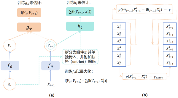
Kaplanis et al. [26] based on the theoretical method of representation learning, use an algorithm to spontaneously learn the macroscopic state variable [math]\displaystyle{ V }[/math] by maximizing [math]\displaystyle{ \mathrm{\Psi} }[/math] (i.e., Equation 1). Specifically, the authors use a neural network [math]\displaystyle{ f_{\theta} }[/math] to learn the representation function that coarsens the microscopic input [math]\displaystyle{ X_t }[/math] into the macroscopic output [math]\displaystyle{ V_t }[/math], and at the same time use neural networks [math]\displaystyle{ g_{\phi} }[/math] and [math]\displaystyle{ h_{\xi} }[/math] to learn the calculation of mutual information such as [math]\displaystyle{ I(V_t;V_{t + 1}) }[/math] and [math]\displaystyle{ \sum_i(I(V_{t + 1};X_{t}^i)) }[/math] respectively. Finally, this method optimizes the neural network by maximizing the difference between the two (i.e., [math]\displaystyle{ \mathrm{\Psi} }[/math]). The architecture diagram of this neural network system is shown in Figure a below.
Figure b shows a toy model example. The microscopic input [math]\displaystyle{ X_t(X_t^1,...,X_t^6) \in \{0,1\}^6 }[/math] has six dimensions, and each dimension has two states of 0 and 1. [math]\displaystyle{ X_{t + 1} }[/math] is the output of [math]\displaystyle{ X_{t} }[/math] at the next moment. The macroscopic state is [math]\displaystyle{ V_{t}=\oplus_{i = 1}^{5}X_t^i }[/math], where [math]\displaystyle{ \oplus_{i = 1}^{5}X_t^i }[/math] represents the result of adding the first five dimensions of the microscopic input [math]\displaystyle{ X_t }[/math] and taking the modulo 2. There is an equal [math]\displaystyle{ \gamma }[/math] probability that the macroscopic states at two consecutive moments are equal ([math]\displaystyle{ p(\oplus_{j = 1..5}X_{t + 1}^j=\oplus_{j = 1..5}X_t^j)= \gamma }[/math]). The sixth dimension of the microscopic input at two consecutive moments has an equal probability of [math]\displaystyle{ \gamma_{extra} }[/math] ([math]\displaystyle{ p(X_{t + 1}^6=X_t^6)= \gamma_{extra} }[/math]).
The results show that in the simple example shown in Figure (b), by maximizing [math]\displaystyle{ \mathrm{\Psi} }[/math] through the model constructed in Figure a, the experiment finds that the learned [math]\displaystyle{ \mathrm{\Psi} }[/math] is approximately equal to the true groundtruth [math]\displaystyle{ \mathrm{\Psi} }[/math], verifying the effectiveness of model learning. This system can correctly judge the occurrence of causal emergence. However, this method also has the problem of being difficult to deal with complex multivariate situations. This is because the number of neural networks on the right side of the figure is proportional to the number of macroscopic and microscopic variable pairs. Therefore, the more the number of microscopic variables (dimensions), the more the number of neural networks will increase proportionally, which will lead to an increase in computational complexity. In addition, this method is only tested on very few cases, so it cannot be scaled up yet. Finally, more importantly, because the network calculates the approximate index of causal emergence and obtains a sufficient but not necessary condition for emergence, the various drawbacks of the above approximate algorithm will be inherited by this method.
Neural Information Compression Method
In recent years, emerging artificial intelligence technologies have overcome a series of major problems. At the same time, machine learning methods are equipped with various carefully designed neural network structures and automatic differentiation technologies, which can approximate any function in a huge function space. Therefore, Zhang Jiang et al. tried to propose a data-driven method based on neural networks to identify causal emergence from time series data [46][40]. This method can automatically extract effective coarse-graining strategies and macroscopic dynamics, overcoming various deficiencies of the Rosas method [37].
In this work, the input is time series data [math]\displaystyle{ (X_1,X_2,...,X_T ) }[/math], and [math]\displaystyle{ X_t\equiv (X_t^1,X_t^2,…,X_t^p ) }[/math], [math]\displaystyle{ p }[/math] represents the dimension of the input data. The author assumes that this set of data is generated by a general stochastic dynamical system:
[math]\displaystyle{ \frac{d X}{d t}=f(X(t), \xi) }[/math]
Here [math]X(t)[/math] is the microscopic state variable, [math]f[/math] is the microscopic dynamics, and [math]\displaystyle{ \xi }[/math] represents the noise in the system dynamics and can model the random characteristics in the dynamical system. However, [math]\displaystyle{ f }[/math] is unknown.
The so-called causal emergence identification problem refers to such a functional optimization problem:
-
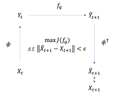
[math]\displaystyle{ \begin{aligned}&\max_{\phi,f_{q},\phi^{\dagger}}\mathcal{J}(f_{q}),\\&s.t.\begin{cases}\parallel\hat{X}_{t + 1}-X_{t + 1}\parallel\lt \epsilon,\\\hat{X}_{t + 1}=\phi^{\dagger}\left(f_{q}(\phi(X_{t})\bigr)\right).\end{cases}\end{aligned} }[/math]
(2)
Here, [math]\mathcal{J}[/math] is the dimension-averaged [math]\displaystyle{ EI }[/math] (see the entry effective information), [math]\displaystyle{ \mathrm{\phi} }[/math] is the coarse-graining strategy function, [math]\displaystyle{ f_{q} }[/math] is the macroscopic dynamics, [math]\displaystyle{ q }[/math] is the dimension of the coarsened macroscopic state, [math]\hat{X}_{t + 1}[/math] is the prediction of the microscopic state at time [math]\displaystyle{ t + 1 }[/math] by the entire framework. This prediction is obtained by performing inverse coarse-graining operation (the inverse coarse-graining function is [math]\phi^{\dagger}[/math]) on the macroscopic state prediction [math]\displaystyle{ \hat{Y}_{t + 1} }[/math] at time [math]\displaystyle{ t + 1 }[/math]. Here [math]\hat{Y}_{t + 1}\equiv f_q(Y_t)[/math] is the prediction of the macroscopic state at time [math]\displaystyle{ t + 1 }[/math] by the dynamics learner according to the macroscopic state [math]Y_t[/math] at time [math]\displaystyle{ t }[/math], where [math]Y_t\equiv \phi(X_t)[/math] is the macroscopic state at time [math]\displaystyle{ t }[/math], which is obtained by coarse-graining [math]X_t[/math] by [math]\phi[/math]. Finally, the difference between [math]\hat{X}_{t + 1}[/math] and the real microscopic state data [math]X_{t + 1}[/math] is compared to obtain the microscopic prediction error.
The entire optimization framework is shown below:
The objective function of this optimization problem is [math]\displaystyle{ EI }[/math], which is a functional of the functions [math]\phi,\hat{f}_q,\phi^{\dagger}[/math] (here the macroscopic dimension [math]q[/math] is a hyperparameter), so it is difficult to optimize. We need to use machine learning methods to try to solve it.
NIS
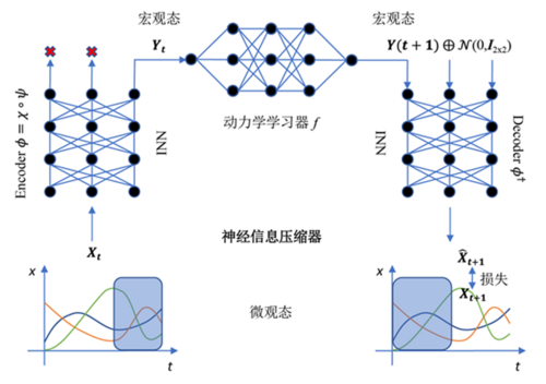
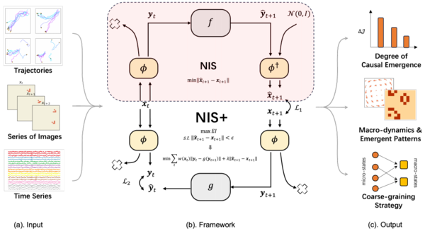
To identify causal emergence in the system, the author proposes a neural information squeezer (NIS) neural network architecture [46]. This architecture is based on an encoder-dynamics learner-decoder framework, that is, the model consists of three parts, which are respectively used for coarse-graining the original data to obtain the macroscopic state, fitting the macroscopic dynamics and inverse coarse-graining operation (decoding the macroscopic state combined with random noise into the microscopic state). Among them, the authors use invertible neural network (INN) to construct the encoder (Encoder) and decoder (Decoder), which approximately correspond to the coarse-graining function [math]\phi[/math] and the inverse coarse-graining function [math]\phi^{\dagger}[/math] respectively. The reason for using invertible neural network is that we can simply invert this network to obtain the inverse coarse-graining function (i.e., [math]\phi^{\dagger}\approx \phi^{-1}[/math]). This model framework can be regarded as a neural information compressor. It puts the microscopic state data containing noise into a narrow information channel, compresses it into a macroscopic state, discards useless information, so that the causality of macroscopic dynamics is stronger, and then decodes it into a prediction of the microscopic state. The model framework of the NIS method is shown in the following figure:
Specifically, the encoder function [math]\phi[/math] consists of two parts:
[math]\displaystyle{ \phi\equiv \chi\circ\psi }[/math]
Here [math]\psi[/math] is an invertible function implemented by an invertible neural network, [math]\chi[/math] is a projection function, that is, removing the last [math]\displaystyle{ p - q }[/math] dimensional components from the [math]\displaystyle{ p }[/math]-dimensional vector. Here [math]\displaystyle{ p,q }[/math] are the dimensions of the microscopic state and macroscopic state respectively. [math]\displaystyle{ \circ }[/math] is the composition operation of functions.
The decoder is the function [math]\phi^{\dagger}[/math], which is defined as:
[math]\displaystyle{ \phi^{\dagger}(y)\equiv \psi^{-1}(y\bigoplus z) }[/math]
Here [math]z\sim\mathcal{Ν}\left (0,I_{p - q}\right )[/math] is a [math]p-q[/math]-dimensional random vector that obeys the standard normal distribution.
However, if we directly optimize the dimension-averaged effective information, there will be certain difficulties. The article [46] does not directly optimize Equation 1, but adopts a clever method. To solve this problem, the author divides the optimization process into two stages. The first stage is to minimize the microscopic state prediction error under the condition of a given macroscopic scale [math]\displaystyle{ q }[/math], that is, [math]\displaystyle{ \min _{\phi, f_q, \phi^{\dagger}}\left\|\phi^{\dagger}(Y(t + 1)) - X_{t + 1}\right\|\lt \epsilon }[/math] and obtain the optimal macroscopic state dynamics [math]f_q^\ast[/math]; the second stage is to search for the hyperparameter [math]\displaystyle{ q }[/math] to maximize the effective information [math]\mathcal{J}[/math], that is, [math]\displaystyle{ \max_{q}\mathcal{J}(f_{q}^\ast) }[/math]. Practice has proved that this method can effectively find macroscopic dynamics and coarse-graining functions, but it cannot truly maximize EI in advance.
In addition to being able to automatically identify causal emergence based on time series data, this framework also has good theoretical properties. There are two important theorems:
Theorem 1: The information bottleneck of the neural information squeezer. That is, for any bijection [math]\displaystyle{ \mathrm{\psi} }[/math], projection [math]\displaystyle{ \chi }[/math], macroscopic dynamics [math]\displaystyle{ f }[/math] and Gaussian noise [math]\displaystyle{ z_{p - q}\sim\mathcal{Ν}\left (0,I_{p - q}\right ) }[/math],
[math]\displaystyle{ I\left(Y_t;Y_{t + 1}\right)=I\left(X_t;{\hat{X}}_{t + 1}\right) }[/math]
always holds. This means that all the information discarded by the encoder is actually noise information unrelated to prediction.
Theorem 2: For a trained model, [math]\displaystyle{ I\left(X_t;{\hat{X}}_{t + 1}\right)\approx I\left(X_t;X_{t + 1}\right) }[/math]. Therefore, combining Theorem 1 and Theorem 2, we can obtain for a trained model:
[math]\displaystyle{ I\left(Y_t;Y_{t + 1}\right)\approx I\left(X_t;X_{t + 1}\right) }[/math]
Comparison with Classical Theories
The NIS framework has many similarities with the computational mechanics framework mentioned in the previous sections. NIS can be regarded as an [math]\displaystyle{ \epsilon }[/math]-machine. The set of all historical processes [math]\displaystyle{ \overleftarrow{S} }[/math] in computational mechanics can be regarded as a microscopic state. All [math]\displaystyle{ R \in \mathcal{R} }[/math] represent macroscopic states. The function [math]\displaystyle{ \eta }[/math] can be understood as a coarse-graining function. [math]\displaystyle{ \epsilon }[/math] can be understood as an effective coarse-graining strategy. [math]\displaystyle{ T }[/math] corresponds to effective macroscopic dynamics. The characteristic of minimum randomness index characterizes the determinism of macroscopic dynamics and can be replaced by effective information in causal emergence. When the entire framework is fully trained and can accurately predict the future microscopic state, the encoded macroscopic state converges to the effective state, and the effective state can be regarded as the causal state in computational mechanics.
At the same time, the NIS framework also has similarities with the G-emergence theory mentioned earlier. For example, NIS also adopts the idea of Granger causality: optimizing the effective macroscopic state by predicting the microscopic state at the next time step. However, there are several obvious differences between these two frameworks: a) In the G-emergence theory, the macroscopic state needs to be manually selected, while in NIS, the macroscopic state is obtained by automatically optimizing the coarse-graining strategy; b) NIS uses neural networks to predict future states, while G-emergence uses autoregressive techniques to fit the data.
Computational Examples
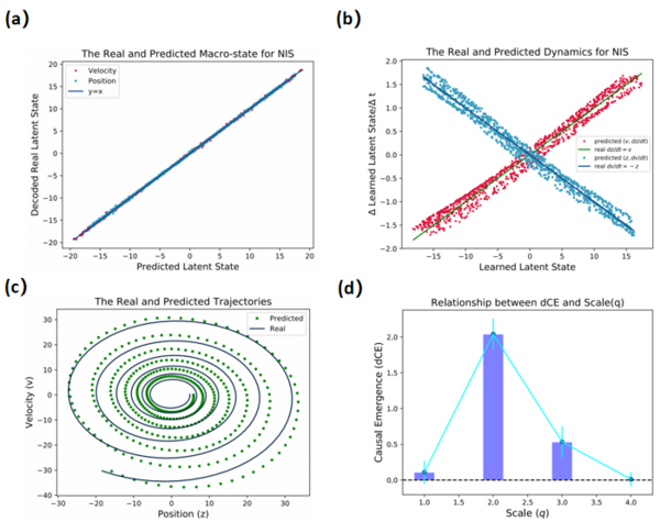
The author of NIS conducted experiments in the spring oscillator model, and the results are shown in the following figure. Figure a shows that the results of encoding at the next moment linearly coincide with the iterative results of macroscopic dynamics, verifying the effectiveness of the model. Figure b shows that the learned two dynamics and the real dynamics also coincide, further verifying the effectiveness of the model. Figure c is the multi-step prediction effect of the model. The prediction and the real curve are very close. Figure d shows the magnitude of causal emergence at different scales. It is found that causal emergence is most significant when the scale is 2, corresponding to the real spring oscillator model. Only two states (position and velocity) are needed to describe the entire system.
NIS+
Although NIS took the lead in proposing a scheme to optimize EI to identify causal emergence in data, this method has some shortcomings: the author divides the optimization process into two stages, but does not truly maximize the effective information, that is, Equation 1. Therefore, Yang Mingzhe et al. [40] further improved this method and proposed the NIS+ scheme. By introducing reverse dynamics and reweighting technique, the original maximization of effective information is transformed into maximizing its variational lower bound by means of variational inequality to directly optimize the objective function.
Mathematical Principles
Specifically, according to variational inequality and inverse probability weighting method, the constrained optimization problem given by Equation 2 can be transformed into the following unconstrained minimization problem:
[math]\displaystyle{ \min_{\omega,\theta,\theta'} \sum_{i = 0}^{T - 1}w(\boldsymbol{x}_t)||\boldsymbol{y}_t-g_{\theta'}(\boldsymbol{y}_{t + 1})||+\lambda||\hat{\boldsymbol{x}}_{t + 1}-\boldsymbol{x}_{t + 1}|| }[/math]
Here [math]\displaystyle{ g }[/math] is the reverse dynamics, which can be approximated by a neural network and trained by the data of [math]y_{t + 1},y_{t}[/math] through the macroscopic state. [math]\displaystyle{ w(x_t) }[/math] is the inverse probability weight, and the specific calculation method is as follows:
[math]\displaystyle{ w(\boldsymbol{x}_t)=\frac{\tilde{p}(\boldsymbol{y}_t)}{p(\boldsymbol{y}_t)}=\frac{\tilde{p}(\phi(\boldsymbol{x}_t))}{p(\phi(\boldsymbol{x}_t))} }[/math]
Here [math]\displaystyle{ \tilde{p}(\boldsymbol{y}_{t}) }[/math] is the target distribution and [math]\displaystyle{ p(\boldsymbol{y}_{t}) }[/math] is the original distribution of the data.
Workflow and Model Architecture
The following figure shows the entire model framework of NIS+. Figure a is the input of the model: time series data, which can be trajectory sequence, continuous image sequence and EEG time series data, etc.; Figure c is the output of the model, including the degree of causal emergence, macroscopic dynamics, emergent patterns and coarse-graining strategies; Figure b is the specific model architecture. Different from the NIS method, two parts of reverse dynamics and reweighting technology are added.
Case Analysis
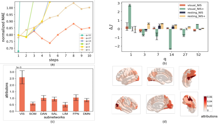
The article conducts experiments on different time series data sets, including the data generated by the disease transmission dynamical system model SIR dynamics, the bird flock model (Boids model) and the cellular automaton: Game of Life, as well as the fMRI signal data of the brain nervous system of real human subjects. Here we choose the bird flock and brain signals for experimental introduction and description.
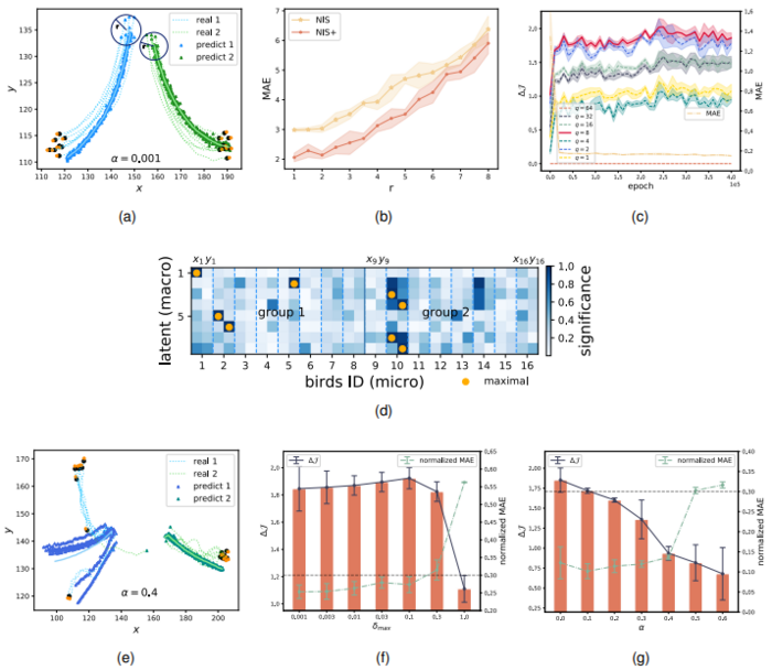
The following figure shows the experimental results of NIS+ learning the flocking behavior of the Boids model. (a) and (e) give the actual and predicted trajectories of bird flocks under different conditions. Specifically, the author divides the bird flock into two groups and compares the multi-step prediction results under different noise levels ([math]\displaystyle{ \alpha }[/math] is 0.001 and 0.4 respectively). The prediction is good when the noise is relatively small, and the prediction curve will diverge when the noise is relatively large. (b) shows that the mean absolute error (MAE) of multi-step prediction gradually increases as the radius r increases. (c) shows the change of causal emergence measure [math]\displaystyle{ \Delta J }[/math] and prediction error (MAE) under different dimensions (q) with the change of training epoch. The author finds that causal emergence is most significant when the macroscopic state dimension q = 8. (d) is the attribution analysis of macroscopic variables to microscopic variables, and the obtained significance map intuitively describes the learned coarse-graining function. Here, each macroscopic dimension can correspond to the spatial coordinate (microscopic dimension) of each bird. The darker the color, the higher the correlation. Here, the microscopic coordinates corresponding to the maximum correlation of each macroscopic state dimension are highlighted with orange dots. These attribution significance values are obtained by using the Integrated Gradient (referred to as IG) method. The horizontal axis represents the x and y coordinates of 16 birds in the microscopic state, and the vertical axis represents 8 macroscopic dimensions. The light blue dotted line distinguishes the coordinates of different individual Boids, and the blue solid line separates the two bird flocks. (f) and (g) represent the changing trends of causal emergence measure [math]\displaystyle{ \Delta J }[/math] and normalized error MAE under different noise levels. (f) represents the influence of changes in external noise (that is, adding observation noise to microscopic data) on causal emergence. (g) represents the influence of internal noise (represented by [math]\displaystyle{ \alpha }[/math], added by modifying the dynamics of the Boids model) on causal emergence. In (f) and (g), the horizontal line represents the threshold that violates the error constraint in Equation 1. When the normalized MAE is greater than the threshold of 0.3, the constraint is violated and the result is unreliable.
This set of experiments shows that NIS+ can learn macroscopic states and coarse-graining strategies by maximizing EI. This maximization enhances the generalization ability of the model to situations beyond the range of training data. The learned macroscopic state effectively identifies the average group behavior and can be attributed to individual positions using the gradient integration method. In addition, the degree of causal emergence increases with the increase of external noise and decreases with the increase of internal noise. This observation result shows that the model can eliminate external noise through coarse-graining, but cannot reduce internal noise.
The brain experiment is based on real fMRI data, which is obtained by performing two sets of experiments on 830 human subjects. In the first group, the subjects were asked to perform a visual task of watching a short movie clip and the recording was completed. In the second group of experiments, they were asked to be in a resting state and the recording was completed. Due to the relatively high original dimension, the authors first reduced the original 14000-dimensional data to 100 dimensions by using the Schaefer atlas method, and each dimension corresponds to a brain region. After that, the authors learned these data through NIS+ and extracted the dynamics at six different macroscopic scales. Figure a shows the multi-step prediction error results at different scales. Figure b shows the comparison of EI of NIS and NIS+ methods on different macroscopic dimensions in the resting state and the visual task of watching movies. The authors found that in the visual task, causal emergence is most significant when the macroscopic state dimension is q = 1. Through attribution analysis, it is found that the visual area plays the largest role (Figure c), which is consistent with the real scene. Figure d shows different perspective views of brain region attribution. In the resting state, one macroscopic dimension is not enough to predict the microscopic time series data. The dimension with the largest causal emergence is between 3 and 7 dimensions.
These experiments show that NIS+ can not only identify causal emergence in data, discover emergent macroscopic dynamics and coarse-graining strategies, but also other experiments show that the NIS+ model can also increase the out-of-distribution generalization ability of the model through EI maximization.
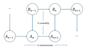
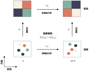

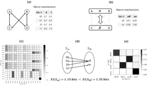
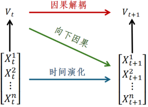

![[math]\displaystyle{ EI }[/math]与[math]\displaystyle{ \Gamma }[/math]对比](/images/thumb/0/03/Gamma%E4%BE%8B%E5%AD%90.png/500px-Gamma%E4%BE%8B%E5%AD%90.png)
