部分信息分解

历史

1948年，克劳德·艾尔伍德·香农（Claude Elwood Shannon）开启了现代信息论研究，为人们提供了分析数据所蕴含信息的强大工具。香农提出的互信息 Mutual Information概念衡量了一个随机变量对另一个随机变量的信息，本词条的核心内容即是建立在此概念之上。经典互信息主要刻画两个随机变量或一个变量组与另一个变量之间的共享信息，但不能直接区分多个源变量对同一目标变量的信息贡献结构。但在现实世界的许多场景中，我们面临的是多个变量之间的相互作用，多变量信息理论应运而生。其中，交互信息 Interaction Information 是被广泛使用的一个概念，其是由熵的容斥原理定义的多变量相关量，混合了冗余与协同，符号可正可负。但信息量显然应该是非负的，这是在面对三个或更多个随机变量时交互信息存在的一个显著的问题，反映了交互信息在解释多变量系统中的局限性。

为了解决这一问题，Paul L. Williams和Randall D. Beer在2010年的论文《多变量信息的非负分解》中提出了一种新的多变量信息分解方式，试图将信息论推广到多个变量的情况。他们重点考虑了一组源变量对目标变量提供信息的一般结构，即将源变量对目标变量提供的信息分成三个部分——冗余，特有，协同以在给定冗余函数后，将源变量组与目标变量的互信息分解为若干部分信息原子。他们的思路是首先给出了冗余 Redundancy的新定义：信息源对每个目标变量的取值提供的最小信息量对所有取值的平均。基于这一定义，他们构建了并引入一个关于源变量集合的冗余晶格 redundancy lattice来阐明多变量信息的一般结构。后利用这个冗余晶格提出了其余两种部分信息原子 Partial Information Atoms（特有信息和协同信息）的定义，并以例子说明了他们构建的部分信息分解 Partial Information Decomposition(简称PID)框架能够将多变量系统中信息源对目标变量提供的贡献分解为信息原子的组合。

相关概念

信息熵

对于一个有[math]\displaystyle{ n }[/math]种可能取值 [math]\displaystyle{ \{x_1,x_2,\dots,x_n\} }[/math]的离散随机变量 [math]\displaystyle{ X }[/math],

每个可能取值对应的概率记为 [math]\displaystyle{ \{p_1,p_2,\dots,p_n\} }[/math]。 度量该随机变量不确定程度的函数[math]\displaystyle{ H(X) }[/math]称为该随机变量的信息熵,[math]\displaystyle{ H(X) }[/math]满足以下三条公理：

1. 连续性：概率的微小变化只会引起不确定度的微小变化,即：[math]\displaystyle{ H(p_1,p_2,\dots,p_n) }[/math]关于[math]\displaystyle{ p_i }[/math]连续。
2. 可加性:若一个随机试验可分解为多个连续的随机试验,那么原随机试验的不确定性应是各不确定性之和。
3. 等概率时单调递增:离散型随机变量所有结果的概率相等时,即[math]\displaystyle{ p_i = \frac{1}{n} }[/math],则[math]\displaystyle{ H }[/math]应是[math]\displaystyle{ n }[/math]的单调递增函数。

通过以上三条公理可确定在常数因子与对数底数之外唯一形式的 [math]\displaystyle{ H(X) }[/math]，形式如下,其中[math]\displaystyle{ K }[/math]为任意常数：

[math]\displaystyle{ H(X) = - K\sum_{i=1}^{n}p_i\log p_i }[/math]

这种公理化思路也在PID框架的构建中得到了应用，PID框架的作者提出冗余信息原子的单调性、上界性、自冗余性公理以约束冗余信息原子的数学形式。

互信息

对多变量系统而言，例如源变量组[math]\displaystyle{ X_1,X_2,\dots X_n }[/math]和一个目标变量[math]\displaystyle{ Y }[/math]之间构成的多变量系统[math]\displaystyle{ \{X_1,X_2,\dots,X_n,Y\} }[/math]，多变量的互信息[math]\displaystyle{ I(X_1,X_2,\dots,X_n;Y) }[/math]被用于描述源变量组[math]\displaystyle{ {X_1,X_2,\dots,X_n} }[/math]对一个目标变量[math]\displaystyle{ Y }[/math]之间传输的信息量[math]\displaystyle{ I(X_1,X_2,\dots,X_n ; Y) }[/math]。

其定义如下:

[math]\displaystyle{ I(X_1,X_2,\dots,X_n ; Y) = I(X_1,X_2,\dots,X_n;Y) = H(X_1,X_2,\dots,X_n)-H(X_1,X_2,\dots,X_n|Y) }[/math]

源变量组对目标变量的传输信息正是PID框架要分解的对象。

在单一源的情形下，两个随机变量的互信息是两个随机变量的相互关联中包含的信息量,其被用于刻画两个随机变量间的关联关系。在百科的后续介绍中我们会看到，不论是总相关性、McGill交互信息，抑或是PID框架，都需要使用信息熵、互信息及条件互信息出发去刻画随机变量间的关联。

设[math]\displaystyle{ X,Y }[/math]为两个离散型随机变量，此情形下两个变量的互信息的定义及计算式为:

[math]\displaystyle{ I(X;Y) =\sum_{i,j}p_{XY}(x_i,y_j)\log_2\left(\frac{p_{XY}(x_i,y_j)}{p_X(x_i)p_{Y}(y_j)}\right) }[/math]

[math]\displaystyle{ =\sum_{i,j}p_{XY}(x_i,y_j)\left(\log_2 p_{XY}(x_i,y_j) - \log_2p_{X}(x_i) - \log_2p_{Y}(y_j)\right) }[/math]

[math]\displaystyle{ = H_X+H_Y - H_{XY} }[/math]

两个变量的互信息可以写成[math]\displaystyle{ (D_{\mathrm{KL}}(p_{XY}\Vert p_Xp_Y)) }[/math]仅度量二元联合分布偏离独立分布的程度；但它不能区分多源情形中的冗余、特有和协同贡献。

条件互信息

对照互信息的意义，可类似地定义条件互信息，条件互信息刻画了有第三方变量的约束情况时，两个变量的关联情况，其定义如下：

设[math]\displaystyle{ X,Y,Z }[/math]为离散型随机变量，条件互信息[math]\displaystyle{ I(X;Y|Z) }[/math]定义为：

[math]\displaystyle{ I(X;Y|Z) = H(X|Z) - H(X|Y,Z) }[/math]

在PID框架原始版本的两源变量情形中，条件互信息将协同信息与特有信息联系了起来。

PID框架的形成动机

在PID框架被提出前，多变量信息理论领域已有两类代表性的信息框架，分别为S. Watanabe于1960提出的总相关性框架及William J. McGill于1954提出的交互信息框架，前者提出的总相关性熵函数为计量多个随机变量集合中交互作用程度的总量提供了计量工具,后者则引出了反直觉的负交互信息问题。这些为PID框架的形成提供了动机，一方面PID框架试图精细量化多变量间传输信息的构成，从而揭示多个随机变量间交互作用的结构特征，另一方面，PID框架要给出交互信息框架中负信息的形成机制及其意义，即为负交互信息问题提供结构化解释。

总相关性

对于给定的[math]\displaystyle{ n }[/math]个随机变量集合

[math]\displaystyle{ \{X_1,X_2,\dots,X_n\} }[/math]

其总相关性[math]\displaystyle{ C(X_1,X_2,\dots,X_n) }[/math]的定义如下：

[math]\displaystyle{ C(X_1,X_2,\dots,X_n) = \sum_{i=1}^{n}H(X_i) - H(X_1,X_2,\dots X_n) }[/math]

其中[math]\displaystyle{ H(X_i) }[/math]是变量的信息熵[math]\displaystyle{ X_i }[/math] ;[math]\displaystyle{ H(X_1,X_2,\dots,X_n) }[/math]为随机变量集合[math]\displaystyle{ H(X_1,X_2,\dots,X_n) }[/math]是变量集[math]\displaystyle{ \{ X_1,X_2,\dots, X_n\} }[/math]的联合熵。

总相关性量化了目标变量集中存在的绝对冗余的总量。但多元随机变量间冗余的关联亦构成了这一概念的局限，因为总相关性中未包含对冗余结构的细致分析——譬如，在下面例子中所展示的高阶冗余交互作用。

例：三变量情形的高阶交互冗余

设[math]\displaystyle{ \{X_1,X_2,X_3\} }[/math]为一三元随机变量组变量组，其中[math]\displaystyle{ X_1,X_2,X_3 }[/math]两两独立，但[math]\displaystyle{ X_1,X_2 }[/math]构成的整体与[math]\displaystyle{ X_3 }[/math]有关联。

一个实例：令[math]\displaystyle{ X_1,X_2,X_3 }[/math]构成了一两输入XOR电路门，[math]\displaystyle{ \{X_1,X_2\} }[/math]为前两个输入的整体输入情况，[math]\displaystyle{ X_3 }[/math]为[math]\displaystyle{ X_1\oplus X_2 }[/math]的输出情况。

[math]\displaystyle{ X_1,X_2,X_3 }[/math]两两独立，但[math]\displaystyle{ \{X_1,X_2\} }[/math]整体的输入情况[math]\displaystyle{ \{X_1,X_2\} }[/math]，和[math]\displaystyle{ X_3 }[/math]的输出情况之间是冗余的。

高阶交互冗余的存在启发了PID框架重新严格定义冗余信息并对传输信息的来源进行分解。

McGill 交互信息

McGill交互信息又称多重互信息或共信息，其定义方式如下：

设[math]\displaystyle{ \mathcal{V}= \{X_1,X_2,\dots,X_n\} }[/math]为一组离散型随机变量构成的集合，它们的McGill交互信息由互信息和条件互信息组成的递归式给出，如下所示

[math]\displaystyle{ I(X_1;X_2;\dots;X_{n+1}) = I(X_1;\dots;X_n) -I(X_1;\dots;X_n|X_{n+1}) }[/math]

当[math]\displaystyle{ I(X_1,X_2,\dots,X_n) }[/math]以随机变量的信息熵和联合熵表达时,可以写成如下形式：

[math]\displaystyle{ I(\mathcal{V}) = \sum_{\tau \subseteq \mathcal{V}} (-1)^{|\tau|-1}H(\tau) }[/math]

其中[math]\displaystyle{ H(\emptyset)=0 }[/math]

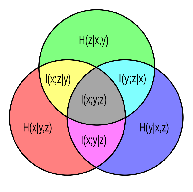
对三元随机变量集合[math]\displaystyle{ \{X,Y,Z\} }[/math]而言，相应的McGill交互信息为下图中的灰色部分:[math]\displaystyle{ I(X;Y;Z) }[/math]

负交互信息问题

对单变量的信息熵而言，信息熵始终是一非负值，但在McGill的交互信息框架中却会出现多变量间交互信息为负值的情况，这种反直觉的事实意味着，McGill的多变量信息框架存在着缺陷，这一问题使得后续的工作者尝试发展更完备的多变量信息理论，PID就是其中一种。

下面的例子展示了McGill交互信息框架中的负信息问题。

设[math]\displaystyle{ X,Y,Z }[/math]为三个离散型随机变量，每个随机变量取值均只有[math]\displaystyle{ \{0,1\} }[/math]两种可能，依次代表汽车启动能启动，汽车发动机的电池能否正常工作，汽车的发动机的燃油泵是否能正常工作。

其中，电池能否正常工作与燃油泵能否正常工作独立,而当且仅当电池和燃油泵同时工作时，车的动力系统[math]\displaystyle{ \{Y,Z\} }[/math]正常运作，车才可以运行，从而[math]\displaystyle{ I(Y;Z) = 0 }[/math]

但车无法启动,电池工作良好，则可推出发动机故障，从而：

[math]\displaystyle{ I(Y;Z|X) \gt 0 }[/math]

此时：

[math]\displaystyle{ I(X;Y;Z) = I(Y;Z) - I(Y;Z|X) \lt 0 }[/math]

McGill交互信息负值的出现意味着本不是冗余的信息被计算成了冗余信息,从而暗示了以往被算作“冗余信息”的部分可能包含着多个变量形成整体间互相作用的效果,启发了PID框架将协同计入信息原子。

部分信息分解（PID）框架

冗余信息的定义

令 [math]\displaystyle{ S_1,S_2,\dots ,S_n }[/math]为 [math]\displaystyle{ \mathbf{S} }[/math]的非空且允许重叠的子集，我们称之为源。每个源[math]\displaystyle{ S_i }[/math]所提供的信息由互信息[math]\displaystyle{ I(T;S_i) }[/math]给出。然而，关键在于互信息实际上是对随机变量的所有可能结果取的平均或期望信息。因此，两个源可能提供相同的平均信息量，同时却关于[math]\displaystyle{ T }[/math]的不同结果提供信息。源[math]\displaystyle{ S }[/math]所提供的信息可写为 \begin{equation} I(T;S)=\sum_{t}p(t)\,I(T=t;S) \end{equation} 其中特定信息[math]\displaystyle{ I(T=t;S) }[/math]量化了与[math]\displaystyle{ T }[/math]的某一特定结果 [math]\displaystyle{ t }[/math]相关联的信息。下面需要给出其定义： \begin{equation} I(T=t;S)= \sum_{s}p(s|t) \left[\log\frac{1}{p(t)}-\log\frac{1}{p(t|s)}\right] \end{equation} 项[math]\displaystyle{ \log1/p(t) }[/math]称为[math]\displaystyle{ t }[/math]的不确定度(surprise)。因此 [math]\displaystyle{ I(T=t;S) }[/math]是在[math]\displaystyle{ T=t }[/math]条件下，对源变量取值[math]\displaystyle{ s\sim p(s|t) }[/math]加权平均的不确定度减少量。这是一种很自然的定义。例如对特定结果[math]\displaystyle{ t }[/math]发生的条件下[math]\displaystyle{ S }[/math]以百分之五十概率取[math]\displaystyle{ s_1 }[/math]，以百分之五十的概率取[math]\displaystyle{ s_2 }[/math]，显然可以用这两个取值对[math]\displaystyle{ t }[/math]的不确定度减少量加权平均来定义平均不确定度减少量（即[math]\displaystyle{ I(T=t;S) }[/math]）。总之，[math]\displaystyle{ I(T=t;S) }[/math] 量化 [math]\displaystyle{ S }[/math]关于每个特定结果 [math]\displaystyle{ t\in T }[/math]所提供的信息，而[math]\displaystyle{ I(T;S) }[/math]则是该量在所有结果上的期望。根据此，一个自然的冗余度量是每个源关于每个结果所提供信息的最小值的期望，即 \begin{equation} I_{\min}(T;\{S_1,S_2,\dots ,S_n\}) =\sum_{t}p(t)\min_{S_i}I(T=t;S_i). \end{equation} [math]\displaystyle{ I_{\min} }[/math]满足了“冗余是所有源共有的信息”这一直觉。同时，特定源的互信息的定义涉及到先对这个源的所有取值求平均再对[math]\displaystyle{ T }[/math]的所有结果求平均两个平均过程，而冗余度的定义中将取最小值这个过程放在第一次平均之后，第二次平均之前是因为不同源可能关于[math]\displaystyle{ T }[/math]的不同结果提供信息。

注：为什么在三种信息里面只给出冗余信息的定义见“冗余晶格”小节第二段。

冗余函数/交集信息的若干公理化性质

根据上述定义可以得到如下关于冗余信息的性质：

非负性：要证明冗余信息是非负的，只需要证明[math]\displaystyle{ I(T=t;S) }[/math]是非负的。我们有[math]\displaystyle{ I(T=t;S)=D(p(s|t)||p(s))\ge 0 \ }[/math] 其中 [math]\displaystyle{ D }[/math]为 Kullback-Leibler 散度。而显然KL散度是非负的。

上界性： 对所有 [math]\displaystyle{ S_i }[/math]都有 [math]\displaystyle{ I_{\min}\le I(T;S_i) }[/math]，且当且仅当对所有 [math]\displaystyle{ i,j }[/math]和所有 [math]\displaystyle{ t\in T }[/math]都有 [math]\displaystyle{ I(T=t;S_i)=I(T=t;S_j) }[/math]时等号成立。

自冗余性: 根据上界性，我们可知

信息量自然地被每个源所提供的信息量上界约束，且当所有源提供完全相同信息时达到该界。此时对给定源 [math]\displaystyle{ S }[/math]，与[math]\displaystyle{ S }[/math]冗余的信息量最大为[math]\displaystyle{ I_{\min}(T;\{S\})=I(T;S) }[/math]。换言之，冗余信息在“自冗余”时候有最大值，这类似于互信息在自信息 [math]\displaystyle{ I(T;T)=H(T) }[/math] 最大化的性质。

下面是交集信息具有的性质（Griffith 2014）:

全局非负性：[math]\displaystyle{ I_\cap(X_1,\dots,X_n:Y)\ge 0 }[/math]。

等价类不变性：对任意 [math]\displaystyle{ i=1,\dots,n }[/math] 或 [math]\displaystyle{ Y }[/math]替换为信息等价随机变量，[math]\displaystyle{ I_\cap(X_1,\dots,X_n:Y) }[/math]保持不变。

目标单调性：若 [math]\displaystyle{ Y\preceq Z }[/math]，则 [math]\displaystyle{ I_\cap(X_1,\dots,X_n:Y)\le I_\cap(X_1,\dots,X_n:Z) }[/math]

弱单调性：对任意额外变量 [math]\displaystyle{ W }[/math]， [math]\displaystyle{ I_\cap(X_1,\dots,X_n,W:Y)\le I_\cap(X_1,\dots,X_n:Y) }[/math]且若存在 [math]\displaystyle{ Z\in\{X_1,\dots,X_n\} }[/math]使得 [math]\displaystyle{ Z\preceq W }[/math]，则等号成立。

弱对称性：[math]\displaystyle{ I_\cap(X_1,\dots,X_n:Y) }[/math] 对 [math]\displaystyle{ X_1,\dots,X_n }[/math]的排列顺序不变。

以下性质将交集信息与所选信息度量 [math]\displaystyle{ \mathcal{I}(X:Y) }[/math] 联系起来：

下界：若随机变量 [math]\displaystyle{ Q }[/math] 满足 [math]\displaystyle{ Q\preceq X_i }[/math] 对所有 [math]\displaystyle{ i=1,\dots,n }[/math]成立，则 [math]\displaystyle{ I_\cap(X_1,\dots,X_n:Y)\ge \mathcal{I}(Q:Y) }[/math]特别地，[math]\displaystyle{ Q=X_1\wedge\cdots\wedge X_n }[/math] 是一个合法选择。由 [math]\displaystyle{ I_\cap(X:Y)=\mathcal{I}(X:Y) }[/math] 及弱单调性可推出本性质。

恒等性： [math]\displaystyle{ I_\cap(X,Y:X\vee Y)=\mathcal{I}(X:Y) }[/math]

弱局部非负性：当 [math]\displaystyle{ n=2 }[/math]时，由Williams和beer（2010）定义的部分信息非负。若全局非负性、弱单调性及 [math]\displaystyle{ I_\cap(X_1,X_2:Y)\ge I(X_1:Y)+I(X_2:Y)-I(X_1\vee X_2:Y) }[/math] 同时成立，则本性质自动满足。

最后，更强的性质如下：

强单调性：对任意额外变量 [math]\displaystyle{ W }[/math]， [math]\displaystyle{ I_\cap(X_1,\dots,X_n,W:Y)\le I_\cap(X_1,\dots,X_n:Y) }[/math] 且若存在 [math]\displaystyle{ Z\in\{X_1,\dots,X_n,Y\} }[/math]使得 [math]\displaystyle{ Z\preceq W }[/math]，则等号成立。

强对称性：[math]\displaystyle{ I_\cap(X_1,\dots,X_n:Y) }[/math] 对 [math]\displaystyle{ X_1,\dots,X_n,Y }[/math]的排列顺序不变。

强局部非负性：对任意 [math]\displaystyle{ n }[/math]，由Williams和beer(2010)定义的部分信息均非负。

两源变量PID框架与部分信息原子

这里,集智百科先以两源变量的情形向各位读者展示部分信息分解（PID）框架中所涉及的核心概念。

两源变量PID框架的基本构成如下：

设有三个随机变量，[math]\displaystyle{ S_1,S_2,T }[/math],其中[math]\displaystyle{ T }[/math]为信道中的目标变量,[math]\displaystyle{ S_1,S_2 }[/math]为信道中的源变量

记[math]\displaystyle{ S_1,S_2 }[/math]整体构成了随机变量组:

[math]\displaystyle{ \mathbf{S} = \{S_1,S_2\} }[/math]

PID框架要分解的是[math]\displaystyle{ \mathbf{S} }[/math]对[math]\displaystyle{ T }[/math]的传递信息[math]\displaystyle{ I(\mathbf{S};T) }[/math].

如下面的韦恩图所示,部分信息分解框架中将[math]\displaystyle{ \mathbf{S} }[/math]对[math]\displaystyle{ T }[/math]的传递信息[math]\displaystyle{ I(\mathbf{S};T) }[/math]为如下三个基本单元,PID框架中,这些基本单元被称为部分信息原子：

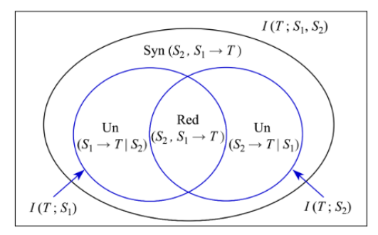
部分信息原子包括如下三个部分:

特有信息(Un):仅源变量[math]\displaystyle{ S_1,S_2 }[/math]中的一个自身可以向[math]\displaystyle{ T }[/math]目标提供,而另一个无法提供的信息。

[math]\displaystyle{ \mathrm{Un}(S_1 \rightarrow T | S_2),\mathrm{Un}(S_2 \rightarrow T| S_1) }[/math]

冗余信息(Red): [math]\displaystyle{ R_1,R_2 }[/math]均可提供的重复信息（冗余信息）

[math]\displaystyle{ \mathrm{Red}(S_1,S_2\rightarrow T) }[/math]

协同信息(Syn):[math]\displaystyle{ R_1,R_2 }[/math]的组合可能产生单独任何一个随机变量无法提供的信息

[math]\displaystyle{ \mathrm{Syn}(S_1,S_2 \rightarrow T) }[/math]

从而有

[math]\displaystyle{ I(\mathbf{S};T)=I((S_1,S_2);T) = \mathrm{Syn}(S_1,S_2 \rightarrow T)+ \mathrm{Un}(S_1 \rightarrow T | S_2)+\mathrm{Un}(S_2 \rightarrow T| S_1)+\mathrm{Red}(S_1,S_2\rightarrow T) }[/math]

从维恩图中显而易见的还有如下两组等式等式成立：

1. 某一源向目标变量传递的信息由其特有和冗余构成

[math]\displaystyle{ I(S_1;T) = \mathrm{Red}(S_1,S_2 \rightarrow T) + \mathrm{Un}(S_1 \rightarrow T| S_2) }[/math]

[math]\displaystyle{ I(S_2;T) = \mathrm{Red}(S_1,S_2 \rightarrow T) + \mathrm{Un}(S_2 \rightarrow T|S_1) }[/math]

这意味着，我们可以通过互信息-冗余去计算特有信息。

2. 某一源向和目标变量组（整体）传递的信息由特有和协同构成

[math]\displaystyle{ I(T;S_1 |S_2) = \mathrm{Syn}(S_1,S_2 \rightarrow T) + \mathrm{Un}(S_1 \rightarrow T |S_2) }[/math]

[math]\displaystyle{ I(T;S_2 |S_1) = \mathrm{Syn}(S_1,S_2 \rightarrow T) + \mathrm{Un}(S_2 \rightarrow T| S_1) }[/math]

这意味着，在通过互信息-冗余计算完特有后，我们可以用条件互信息-特有计算协同。

在此，集智百科将先以两源变量框架为例，展示信息原子的计算过程，为了在后面的例子中进行计算，这里先给出两源变量情形下冗余信息的计算式。依照Paul L. Williams和Randall D. Beer在论文中给出一般定义，容易得到冗余信息在两源变量框架中的计算式：

[math]\displaystyle{ \mathrm{Red}(S_1,S_2 \rightarrow T) =I(T=t;S_i)=\sum_{s_i}p(s_i|t)\log_2\frac{p(t|s_i)}{p(t)} }[/math]

其中

[math]\displaystyle{ I(T = t; S_i) = \sum_{\mathbf{s}}p(\mathbf{\mathbf{s}}|t)\log_2\frac{p(t|\mathbf{s})}{p(\mathbf{s})} }[/math]

在给出两源情形下的冗余信息原子的定义后，集智百科将以经典的异或目标变量情形为例展示PID的计算过程，并同时计算总相关性与McGill交互信息，讨论PID框架如何解释McGill交互信息的负值问题。

例：

[math]\displaystyle{ X,Y,Z }[/math]三元变量组中，设[math]\displaystyle{ X,Y }[/math]独立,[math]\displaystyle{ Z =X \oplus Y }[/math]

本例中，当[math]\displaystyle{ X,Y,Z }[/math]的分布及相应的联合分布按下方表格中的方式给出时，可以相应的计算出该两源随机变量系统中熵、条件熵、相应的条件互信息，从而获得这组随机变量的总相关性、McGill交互信息。

又由[math]\displaystyle{ X,Y }[/math]间的独立性可知[math]\displaystyle{ \mathrm{Red}(X,Y,→ Z) = 0 }[/math],又由异或逻辑的构造和[math]\displaystyle{ X,Y,Z }[/math]间的两两独立性知[math]\displaystyle{ \mathrm{Syn}(X,Y \rightarrow Z) \neq 0 }[/math]，可大致了传输信息是如何在这组变量的信息原子之间的分布情况。

[math]\displaystyle{ X }[/math]	[math]\displaystyle{ 0 }[/math]	[math]\displaystyle{ 1 }[/math]
[math]\displaystyle{ p_{X} }[/math]	[math]\displaystyle{ \frac{1}{2} }[/math]	[math]\displaystyle{ \frac{1}{2} }[/math]
[math]\displaystyle{ Y }[/math]	[math]\displaystyle{ 0 }[/math]	[math]\displaystyle{ 1 }[/math]
[math]\displaystyle{ p_Y }[/math]	[math]\displaystyle{ \frac{1}{2} }[/math]	[math]\displaystyle{ \frac{1}{2} }[/math]
[math]\displaystyle{ Z=X \oplus Y }[/math]	[math]\displaystyle{ 0 }[/math]	[math]\displaystyle{ 1 }[/math]
[math]\displaystyle{ p_{Z} }[/math]	[math]\displaystyle{ \frac{1}{2} }[/math]	[math]\displaystyle{ \frac{1}{2} }[/math]

[math]\displaystyle{ (X,Y) }[/math]	[math]\displaystyle{ p_{XY} }[/math]	[math]\displaystyle{ p_Xp_Y }[/math]
[math]\displaystyle{ (0,0) }[/math]	[math]\displaystyle{ \frac{1}{4} }[/math]	[math]\displaystyle{ \frac{1}{4} }[/math]
[math]\displaystyle{ (0,1) }[/math]	[math]\displaystyle{ \frac{1}{4} }[/math]	[math]\displaystyle{ \frac{1}{4} }[/math]
[math]\displaystyle{ (1,0) }[/math]	[math]\displaystyle{ \frac{1}{4} }[/math]	[math]\displaystyle{ \frac{1}{4} }[/math]
[math]\displaystyle{ (1,1) }[/math]	[math]\displaystyle{ \frac{1}{4} }[/math]	[math]\displaystyle{ \frac{1}{4} }[/math]
[math]\displaystyle{ (Y,Z) }[/math]	[math]\displaystyle{ p_{YZ} }[/math]	[math]\displaystyle{ p_Yp_Z }[/math]
[math]\displaystyle{ (0,0) }[/math]	[math]\displaystyle{ \frac{1}{4} }[/math]	[math]\displaystyle{ \frac{1}{4} }[/math]
[math]\displaystyle{ (0,1) }[/math]	[math]\displaystyle{ \frac{1}{4} }[/math]	[math]\displaystyle{ \frac{1}{4} }[/math]
[math]\displaystyle{ (1,0) }[/math]	[math]\displaystyle{ \frac{1}{4} }[/math]	[math]\displaystyle{ \frac{1}{4} }[/math]
[math]\displaystyle{ (1,1) }[/math]	[math]\displaystyle{ \frac{1}{4} }[/math]	[math]\displaystyle{ \frac{1}{4} }[/math]
[math]\displaystyle{ (X,Z) }[/math]	[math]\displaystyle{ p_{XZ} }[/math]	[math]\displaystyle{ p_Xp_Z }[/math]
[math]\displaystyle{ (0,0) }[/math]	[math]\displaystyle{ \frac{1}{4} }[/math]	[math]\displaystyle{ \frac{1}{4} }[/math]
[math]\displaystyle{ (0,1) }[/math]	[math]\displaystyle{ \frac{1}{4} }[/math]	[math]\displaystyle{ \frac{1}{4} }[/math]
[math]\displaystyle{ (1,0) }[/math]	[math]\displaystyle{ \frac{1}{4} }[/math]	[math]\displaystyle{ \frac{1}{4} }[/math]
[math]\displaystyle{ (1,1) }[/math]	[math]\displaystyle{ \frac{1}{4} }[/math]	[math]\displaystyle{ \frac{1}{4} }[/math]

[math]\displaystyle{ (X,Y,Z) }[/math]	[math]\displaystyle{ p_{XYZ} }[/math]	[math]\displaystyle{ p_Xp_Yp_Z }[/math]
[math]\displaystyle{ (0,0,0) }[/math]	[math]\displaystyle{ \frac{1}{4} }[/math]	[math]\displaystyle{ \frac{1}{8} }[/math]
[math]\displaystyle{ (0,1,1) }[/math]	[math]\displaystyle{ \frac{1}{4} }[/math]	[math]\displaystyle{ \frac{1}{8} }[/math]
[math]\displaystyle{ (1,0,1) }[/math]	[math]\displaystyle{ \frac{1}{4} }[/math]	[math]\displaystyle{ \frac{1}{8} }[/math]
[math]\displaystyle{ (1,1,0) }[/math]	[math]\displaystyle{ \frac{1}{4} }[/math]	[math]\displaystyle{ \frac{1}{8} }[/math]

可能的子集类型	集合基数	符号	熵（bit）
[math]\displaystyle{ \{X\} }[/math]	[math]\displaystyle{ 1 }[/math]	+	[math]\displaystyle{ 1 }[/math]
[math]\displaystyle{ \{Y\} }[/math]	[math]\displaystyle{ 1 }[/math]	+	[math]\displaystyle{ 1 }[/math]
[math]\displaystyle{ \{Z\} }[/math]	[math]\displaystyle{ 1 }[/math]	+	[math]\displaystyle{ 1 }[/math]
[math]\displaystyle{ \{X,Y\} }[/math]	[math]\displaystyle{ 2 }[/math]	-	[math]\displaystyle{ 2 }[/math]
[math]\displaystyle{ \{Y,Z\} }[/math]	[math]\displaystyle{ 2 }[/math]	-	[math]\displaystyle{ 2 }[/math]
[math]\displaystyle{ \{X,Z\} }[/math]	[math]\displaystyle{ 2 }[/math]	-	[math]\displaystyle{ 2 }[/math]
[math]\displaystyle{ \{X,Y,Z\} }[/math]	[math]\displaystyle{ 3 }[/math]	+	[math]\displaystyle{ 2 }[/math]

总相关性[math]\displaystyle{ C(X,Y,Z) }[/math]	McGill交互信息[math]\displaystyle{ I(X;Y;Z) }[/math]
[math]\displaystyle{ 1 }[/math]	[math]\displaystyle{ -1 }[/math]

事件	条件熵	条件互信息
[math]\displaystyle{ (X\vert Y) }[/math]	[math]\displaystyle{ 1 }[/math]	[math]\displaystyle{ I(X;Z\vert Y) }[/math]
[math]\displaystyle{ (X\vert Y,Z) }[/math]	[math]\displaystyle{ 0 }[/math]	[math]\displaystyle{ 1 }[/math]
[math]\displaystyle{ (Y\vert X) }[/math]	[math]\displaystyle{ 1 }[/math]	[math]\displaystyle{ I(Y;Z\vert X) }[/math]
[math]\displaystyle{ (Y\vert X,Z) }[/math]	[math]\displaystyle{ 0 }[/math]	[math]\displaystyle{ 1 }[/math]

其中，依定义易求得:

[math]\displaystyle{ \mathrm{Red}(S_1,S_2 \rightarrow T) = 0 }[/math]

而可进一步计算:计算PID框架下相应的特有[math]\displaystyle{ \mathrm{Un}(X\rightarrow Z|Y),\mathrm{Un}(Y\rightarrow Z|X) }[/math]与协同[math]\displaystyle{ \mathrm{Syn}(X,Y \rightarrow Z) }[/math]这两种信息原子。

[math]\displaystyle{ \mathrm{Un}(X\rightarrow Z|Y) = \mathrm{Un}(Y\rightarrow Z|X) = -\mathrm{Red}(X,Y \rightarrow Z) =0 }[/math]

[math]\displaystyle{ \mathrm{Syn}(X,Y \rightarrow Z) = I(T;S_1 |S_2) = I(T;S_2 |S_1) =1 }[/math]

容易验证，此时，该三变量系统分解所得的冗余-协同[math]\displaystyle{ =0-1 =-1 }[/math]，即是McGill交互信息的值。

从PID的两源变量框架的算例中可知，若想清楚地分解源变量组与目标变量间的传输信息结构，需要先分析清楚冗余;对于冗余结构更为复杂的多元变量情形，PID框架的作者发展出了相应的冗余晶格理论。

冗余晶格

在上面的两源变量的维恩图里我们可以观察到：

[math]\displaystyle{ I(T;S_{1})=Unq(T;S_{1})+Rdn(T;S_{1},S_{2}) }[/math]

[math]\displaystyle{ I(T;S_{1},S_{2})=Unq(T;S_{1})+Rdn(T;S_{1},S_{2})+Unq(T;S_{2})+Syn(T;S_{1},S_{2}) }[/math]

由于[math]\displaystyle{ I(T;S_{1}) }[/math]和[math]\displaystyle{ I(T;S_{2}) }[/math]和[math]\displaystyle{ I(T;S_{1},S_{2}) }[/math]都是已知的，则我们给定冗余信息，协同信息，特有信息中任何一个的定义都可以唯一确定这个两源变量的系统，PID框架的原始论文中选了冗余信息。基于下述三大冗余信息公理可以得到冗余信息的定义。

但对于多源变量的情况，其协同信息，特有信息，冗余信息（即部分信息原子）结构十分复杂，难以直接进行分解。因此，我们需要使用冗余晶格来重塑系统的结构以产生一个偏序关系使其可以通过莫比乌斯反演得到类似上一段里的两源变量部分信息分解的关系式，再结合冗余信息的定义得到每个部分信息原子。下面介绍冗余晶格如何产生。

在维恩图中，冗余度可以视为[math]\displaystyle{ I（T;S_i) }[/math]之间的交集。因此通过集合之间的包含关系，我们可以大大简化冗余度的概念 举例而言，考虑两个源[math]\displaystyle{ \mathbf{A} }[/math]与[math]\displaystyle{ \mathbf{B} }[/math]，且 [math]\displaystyle{ \mathbf{A}\subseteq\mathbf{B} }[/math]。 显然，[math]\displaystyle{ \mathbf{A} }[/math] 提供的任何信息也被[math]\displaystyle{ \mathbf{B} }[/math]提供，因此 [math]\displaystyle{ \mathbf{A} }[/math]与[math]\displaystyle{ \mathbf{B} }[/math]之间的冗余退化为[math]\displaystyle{ \mathbf{A} }[/math]的自冗余： \begin{equation} I_{\min}(S;\{\mathbf{A},\mathbf{B}\}) =I_{\min}(S;\{\mathbf{A}\})=I(S;\mathbf{A}). \end{equation} 进一步，对任意源[math]\displaystyle{ \mathbf{C} }[/math]，有[math]\displaystyle{ I_{\min}(S;\{\mathbf{A},\mathbf{B},\mathbf{C}\}) =I_{\min}(S;\{\mathbf{A},\mathbf{C}\}) }[/math]。 推广之，对于任何源集合，若其中某些源是其他源的超集（即这个源包含其他源），则该集合的冗余等价于去掉所有超集后的冗余。因此，[math]\displaystyle{ I_{\min} }[/math]的定义域可简化为无源是其他源的超集的那些集合。即： \begin{equation} \mathcal{A}(S)= \bigl\{\alpha\in\mathcal{P}_{1}(\mathcal{P}_{1}(S)) \mid \forall S_i,S_j\in\alpha,\; S_i\not\subset S_j \bigr\}, \end{equation} 其中 [math]\displaystyle{ \mathcal{P}_{1}(S)=\mathcal{P}(S)\setminus\{\emptyset\} }[/math]为[math]\displaystyle{ S }[/math]的所有非空子集的集合。 此后，我们将用带括号的索引简记[math]\displaystyle{ \mathcal{A}(\mathbf{R}) }[/math]的元素，例如： [math]\displaystyle{ \{\{R_{1},R_{2}\}\} }[/math]记为[math]\displaystyle{ \{12\} }[/math]，[math]\displaystyle{ \{\{R_{1}\},\{R_{2}，R_{3}\}\} }[/math]记为[math]\displaystyle{ \{1\}\{23\} }[/math] 通过将上述思路进一步延伸，可在[math]\displaystyle{ \mathcal{A}(\mathbf{R}) }[/math]的元素上定义一个偏序[math]\displaystyle{ \preccurlyeq }[/math]。 考虑两个源集合 [math]\displaystyle{ \alpha,\beta\in\mathcal{A}(\mathbf{R}) }[/math]，若对每个源 [math]\displaystyle{ \mathbf{B}\in\beta }[/math] 都存在源[math]\displaystyle{ \mathbf{A}\in\alpha }[/math]使得 [math]\displaystyle{ \mathbf{A}\subseteq\mathbf{B} }[/math]，则意味着 [math]\displaystyle{ \beta }[/math]中所有源所共享的冗余信息至少包含[math]\displaystyle{ \alpha }[/math]中所有源所共享的冗余信息。 于是，我们可定义偏序： \begin{equation} \forall\alpha,\beta\in\mathcal{A}(\mathbf{R}),\quad \alpha\preccurlyeq\beta \;\Longleftrightarrow\; \forall\mathbf{B}\in\beta,\; \exists\mathbf{A}\in\alpha,\; \mathbf{A}\subseteq\mathbf{B}. \end{equation} 将此偏序应用于[math]\displaystyle{ \mathcal{A}(\mathbf{R}) }[/math]的元素，便得到冗余晶格（redundancy lattice）(见下图展示了三源变量的冗余晶格结构和其对应的韦恩图)，该偏序给出了不同反链之间的包含关系；冗余函数在该偏序上是单调的，进而可通过莫比乌斯反演定义部分信息原子。

下面，集智百科将介绍构建三源变量的冗余晶格的思路：

首先图中的节点含义类比两源变量系统可做如下近似理解（注：这些节点可在两源变量系统中直观对应特有、冗余、协同成分，但在三源以上不能简单逐字解释为某一种日常意义上的信息类型）：特有信息： [math]\displaystyle{ \{1\}, \{2\}, \{3\} }[/math] ；两变量间的冗余信息： [math]\displaystyle{ \{1\}\{2\}, \{1\}\{3\}, \{2\}\{3\} }[/math]）；两变量间的协同信息： [math]\displaystyle{ \{12\}, \{13\}, \{23\} }[/math]。所有三个变量共同提供的冗余信息： [math]\displaystyle{ \{1\}\{2\}\{3\} }[/math]；所有三个变量共同提供的协同信息： [math]\displaystyle{ \{123\} }[/math]；一个变量单独提供的信息，与另外两个变量联合提供的信息之间存在的冗余信息： [math]\displaystyle{ \{1\}\{23\} }[/math]、[math]\displaystyle{ \{2\}\{13\} }[/math] 和 [math]\displaystyle{ \{3\}\{12\} }[/math] ；三个两两协同的信息之间存在的冗余信息 ：[math]\displaystyle{ \{12\}\{13\}\{23\} }[/math] ；变量12的协同信息和变量23的协同信息间存在的冗余信息：[math]\displaystyle{ \{12\}\{23\} }[/math]。

然后，节点间的连边代表了一种邻接关系。最后，我们可以从三个变量共同提供的冗余信息放在最下层开始，比这个区域多一些信息的区域是两变量间的冗余信息，将这些节点放在上一层并且由于这些节点均来自最底层节点添加了一些信息（即按照上述偏序关系找到这个偏序里比这个区域能提供更多信息的下一个或多个区域），故这三个节点都与最底层的节点间有邻接关系（连边），对节点[math]\displaystyle{ \{12\} }[/math]再添加一些信息可以得到节点 [math]\displaystyle{ \{1\}\{23\} }[/math]、[math]\displaystyle{ \{2\}\{13\} }[/math]故这两个节点与节点[math]\displaystyle{ \{12\} }[/math]间有连边。以此类推可以得到完整的三源变量冗余晶格。

这里我们可以发现，这个偏序关系实际上找到了一个基于冗余的对图1中结构的重塑。原本的结构是先有两个源变量分别提供的互信息和两个源变量共同提供的互信息[math]\displaystyle{ I(S;R_{1}) }[/math]，[math]\displaystyle{ I(S;R_{2}) }[/math]和[math]\displaystyle{ I(S;R_{1},R_{2}) }[/math]然后通过对其的分类产生了[math]\displaystyle{ Unq(S;R_{1}) }[/math]，[math]\displaystyle{ Rdn(S;R_{1},R_{2}) }[/math]，[math]\displaystyle{ Unq(S;R_{2}) }[/math]，[math]\displaystyle{ Syn(S;R_{1},R_{2});\{1\}) }[/math]。重塑后的结构将[math]\displaystyle{ I(S;R_{1}) }[/math]和[math]\displaystyle{ I(S;R_{2}) }[/math]理解为其的自冗余将[math]\displaystyle{ I(S;R_{1},R_{2}) }[/math]理解为其的自冗余，并以[math]\displaystyle{ Rdn(S;R_{1},R_{2}) }[/math]为提供最少信息的一种基，在其上逐层添加提供更多信息来产生出[math]\displaystyle{ I(S;R_{1}) }[/math]，[math]\displaystyle{ I(S;R_{2}) }[/math]和[math]\displaystyle{ I(S;R_{1},R_{2}) }[/math]，即形成冗余晶格，其又构成了下文通过累积信息函数得到对交互信息的分解的基础。

其余信息原子计算

冗余晶格中每个节点所关联的冗余信息，不仅包含所有低于它的节点所提供的冗余信息，还可能包含更多。因此，沿着冗余晶格从下到上移动,[math]\displaystyle{ I_{\min} }[/math]可视为一种“累积信息函数”，它对越来越大，越来越包容的源集合所提供的信息进行累积。根据上述，两源变量的情况下我们很容易将交互信息分解为基本信息原子（即特有，冗余，协同三部分）并计算出其具体值，但对多个源变量我们需要使用[math]\displaystyle{ I_{\min} }[/math]的一个逆函数，称为部分信息函数（PI-function）来找到基本信息原子。对于源集合[math]\displaystyle{ \alpha\in\mathcal{A}(\mathbf{R}) }[/math]，部分信息函数记为[math]\displaystyle{ \Pi_{\mathbf{R}} }[/math]，并由下式定义： \begin{equation} I_{\min}(S;\alpha) =\sum_{\beta\preccurlyeq\alpha}\Pi_{\mathbf{R}}(S;\beta). \end{equation} 形式上，[math]\displaystyle{ \Pi_{\mathbf{R}} }[/math] 对应于[math]\displaystyle{ I_{\min} }[/math]的莫比乌斯反演。由该关系可递归计算[math]\displaystyle{ \Pi_{\mathbf{R}} }[/math]： \begin{equation} \Pi_{\mathbf{R}}(S;\alpha) =I_{\min}(S;\alpha) -\sum_{\beta\prec\alpha}\Pi_{\mathbf{R}}(S;\beta). \end{equation} 换言之，[math]\displaystyle{ \Pi_{\mathbf{R}}(S;\alpha) }[/math]量化的是：[math]\displaystyle{ \alpha }[/math]中所有源共同提供的冗余信息中，未被任何比 [math]\displaystyle{ \alpha }[/math]更低的源集合 [math]\displaystyle{ \beta }[/math]所提供的那部分信息。互信息分解为部分信息项之和的关系由下式给出： \begin{equation} I(S;\mathbf{A}) =I_{\min}(S;\{\mathbf{A}\}) =\sum_{\beta\preccurlyeq\{\mathbf{A}\}}\Pi_{\mathbf{R}}(S;\beta). \end{equation} 对于两源变量情形[math]\displaystyle{ \mathbf{R}=\{R_{1},R_{2}\} }[/math]，[math]\displaystyle{ I(S;R_{1})=\Pi_{\mathbf{R}}(S;\{1\})+\Pi_{\mathbf{R}}(S;\{1\}\{2\}) }[/math],[math]\displaystyle{ I(S;R_{1},R_{2})=\Pi_{\mathbf{R}}(S;\{1\})+\Pi_{\mathbf{R}}(S;\{2\})+\Pi_{\mathbf{R}}(S;\{1\}\{2\})+\Pi_{\mathbf{R}}(S;\{12\}) }[/math]。与上文对比，可立即看出每个部分信息项的含义：冗余信息：[math]\displaystyle{ \Pi_{\mathbf{R}}(S;\{1\}\{2\})=I_{\min}(S;\{1\}\{2\}) }[/math]，即 [math]\displaystyle{ R_{1} }[/math]与 [math]\displaystyle{ R_{2} }[/math]的冗余。特有信息：[math]\displaystyle{ \Pi_{\mathbf{R}}(S;\{1\})=I(S;R_{1})-I_{\min}(S;\{1\}\{2\}) }[/math]，即 [math]\displaystyle{ R_{1} }[/math]的总信息减去冗余部分；对 [math]\displaystyle{ R_{2} }[/math]同理。协同信息：[math]\displaystyle{ \Pi_{\mathbf{R}}(S;\{12\}) }[/math] 表示 [math]\displaystyle{ R_{1} }[/math]与 [math]\displaystyle{ R_{2} }[/math]联合后多出来的那部分信息，即协同。

其余信息原子计算实例

为了更具体地理解这些概念，我们来看上图中的例子。由于该分布具有对称性，显然 [math]\displaystyle{ R_1 }[/math] 和 [math]\displaystyle{ R_2 }[/math] 提供的信息量是相同的。实际上，可以验证：

[math]\displaystyle{ I(S;R_1) = I(S;R_2) = - \frac{1}{3} \log \frac{1}{3} - \frac{2}{3} \log \frac{2}{3} }[/math]

(但也可以清楚地看到，[math]\displaystyle{ R_1 }[/math] 和 [math]\displaystyle{ R_2 }[/math] 提供的是关于不同结果的信息。具体来说，只要知道 [math]\displaystyle{ R_1 }[/math] 的值，就可以完全确定结果 [math]\displaystyle{ S=2 }[/math] 是否发生（而 [math]\displaystyle{ R_2 }[/math] 无法做到这一点），反之亦然。)

另外我们有[math]\displaystyle{ I(S;R_1,R_2) = \log 3 }[/math]根据这两个式子及上一小节给出的关系式可以得到如下结果：

[math]\displaystyle{ \Pi_{\mathbf{R}}(S;\{1\}) = \Pi_{\mathbf{R}}(S;\{2\}) = \frac{1}{3} }[/math]，表示 [math]\displaystyle{ R_1 }[/math] 和 [math]\displaystyle{ R_2 }[/math] 各自提供了 [math]\displaystyle{ \frac{1}{3} }[/math] 比特的特有信息；

冗余信息为 [math]\displaystyle{ \Pi_{\mathbf{R}}(S;\{1\}\{2\}) = \log 3 - \log 2 }[/math]，表示知道 [math]\displaystyle{ R_1 }[/math] 或 [math]\displaystyle{ R_2 }[/math] 中的任意一个，都能将 [math]\displaystyle{ S }[/math] 的可能结果从3个减少到2个；

协同信息为 [math]\displaystyle{ \Pi_{\mathbf{R}}(S;\{12\}) = \frac{1}{3} }[/math]，表示 [math]\displaystyle{ R_1 }[/math] 和 [math]\displaystyle{ R_2 }[/math]联合起来可以唯一确定 [math]\displaystyle{ S=0 }[/math] 是否发生，而单独任意一个都无法做到这一点。

（需要注意的是，与互信息或交互信息不同，部分信息分解是相对于选定目标变量的分解，因此交换源变量与目标变量一般会得到不同分解，例如，[math]\displaystyle{ R_1 }[/math] 和 [math]\displaystyle{ R_2 }[/math] 关于 [math]\displaystyle{ S }[/math] 的协同信息，通常不等于 [math]\displaystyle{ S }[/math] 和 [math]\displaystyle{ R_2 }[/math] 关于 [math]\displaystyle{ R_1 }[/math] 的协同信息。这一性质在上面的例子中也得到了体现：一旦知道了 [math]\displaystyle{ S }[/math] 的值，就可以唯一确定 [math]\displaystyle{ R_1 }[/math] 和 [math]\displaystyle{ R_2 }[/math] 的结果，因此不可能存在 [math]\displaystyle{ S }[/math] 和 [math]\displaystyle{ R_2 }[/math] 联合提供关于 [math]\displaystyle{ R_1 }[/math] 的协同信息，因为 [math]\displaystyle{ R_1 }[/math] 的不确定性已经被 [math]\displaystyle{ S }[/math]完全消除了。相反，如前所述，[math]\displaystyle{ R_1 }[/math] 和 [math]\displaystyle{ R_2 }[/math] 却提供了关于 [math]\displaystyle{ S }[/math] 的协同信息。这种不对称性也解释了为什么部分信息分解始终聚焦于关于某个特定变量 [math]\displaystyle{ S }[/math] 的信息，因为在一般情况下，分析的结果会依赖于我们关注的是哪个变量。）

冗余信息计算方法

以下是一些有代表性的定量方法： 首先，第一个定义即原论文给出的定义（见冗余信息定义小节）。

Griffith 基于共同随机变量的交集信息

Griffith 等基于 Gács–Körner common random variable 提出交集信息，原论文构建冗余晶格的方式如下：给定随机变量 [math]\displaystyle{ X }[/math]和 [math]\displaystyle{ Y }[/math]，记 [math]\displaystyle{ X\preceq Y }[/math] 表示存在可测函数 [math]\displaystyle{ f }[/math] 使得 [math]\displaystyle{ X=f(Y) }[/math] 几乎必然成立。此时称 [math]\displaystyle{ X }[/math]在信息上“贫于”[math]\displaystyle{ Y }[/math](informationally poorer），据此可以引入偏序关系。给定随机变量 [math]\displaystyle{ X,Y }[/math]，定义其 join（连接）[math]\displaystyle{ X\vee Y }[/math]为信息上最“贫”的随机变量，使得[math]\displaystyle{ X\preceq X\vee Y }[/math] 且 [math]\displaystyle{ Y\preceq X\vee Y }[/math]；类似地，定义 meet（相遇）[math]\displaystyle{ X\wedge Y }[/math] 为信息上最“富”的随机变量，使得[math]\displaystyle{ X\wedge Y\preceq X }[/math] 且 [math]\displaystyle{ X\wedge Y\preceq Y }[/math]。称 [math]\displaystyle{ X\wedge Y }[/math] 为 [math]\displaystyle{ X }[/math]与 [math]\displaystyle{ Y }[/math]的共同随机变量。

共同随机变量的熵即[math]\displaystyle{ \mathcal{I}=I^0 }[/math]（零误差信息）。对于零误差信息 [math]\displaystyle{ \mathcal{I}=I^0 }[/math]，研究者们提出零误差交集信息[math]\displaystyle{ I_{\cap}^0(X_1,\dots,X_n:Y) }[/math]：它是一个随机变量[math]\displaystyle{ Q }[/math]关于[math]\displaystyle{ Y }[/math]的最大零误差信息 [math]\displaystyle{ I^0(Q:Y) }[/math]，且 Q 是每个源变量 [math]\displaystyle{ X_1,\dots,X_n }[/math]的函数:

[math]\displaystyle{ I_{\cap}^0(X_1,\dots,X_n:Y)\triangleq \max_{\Pr(Q|Y)}I^0(Q:Y)\quad\text{subject to}\quad Q\preceq X_i\; \forall i\in\{1,\dots,n\}. }[/math]

上式可简化为：

[math]\displaystyle{ I_{\cap}^0(X_1,\dots,X_n:Y) =I^0(X_1\wedge\cdots\wedge X_n:Y) =H(X_1\wedge\cdots\wedge X_n\wedge Y). }[/math]

与香农互信息不同其只适用于零误差通信故要改进以适配互信息的场景因此更改为

[math]\displaystyle{ I_{\cap}(X_1,\dots,X_n:Y) =I(X_1\wedge\cdots\wedge X_n:Y). }[/math]

Lyu–Clark–Raviv 显式两源 PID 公式

Lyu 等（2024）受 Pearl do-calculus 启发引入 do-operation（固定某边际的同时最小化对其他条件分布的扰动），首次给出满足 Williams–Beer公理及后续性质的两源部分信息分解的显式公式，而不是任意多源部分信息分解的完整封闭形式冗余晶格解。为了给出信息原子的定义，研究者们构造了一个新的分布（以下所有包含[math]\displaystyle{ S_1' }[/math]的信息量均在该构造分布下计算），如下所示。给定一个包含源变量 [math]\displaystyle{ S_1, S_2 }[/math] 和目标变量 [math]\displaystyle{ T }[/math] 的系统，其相应的字母表分别为 [math]\displaystyle{ \mathcal{S}_1, \mathcal{S}_2 }[/math]和 [math]\displaystyle{ \mathcal{T} }[/math]，研究者们定义一个新的随机变量[math]\displaystyle{ S_1' }[/math] 在[math]\displaystyle{ \mathcal{S}_1 }[/math] 上，通过其条件联合分布如下：

[math]\displaystyle{ \operatorname{Pr}(S_1' = s_1, S_2 = s_2 | T = t) \triangleq \operatorname{Pr}(S_1 = s_1 | T = t) \operatorname{Pr}(S_2 = s_2 | T = t). }[/math]

这意味着，对于每一个[math]\displaystyle{ s_1 \in \mathcal{S}_1 }[/math]，

[math]\displaystyle{ \operatorname{Pr}(S_1' = s_1) = \sum_{(s_2, t) \in \mathcal{S}_2 \times \mathcal{T}} \operatorname{Pr}(S_1 = s_1 | T = t) \operatorname{Pr}(S_2 = s_2 | T = t) \operatorname{Pr}(T = t). }[/math]

变量 [math]\displaystyle{ S_1' }[/math]是良定义的，因为所有概率都是非负的，并且可以很容易地证明：

[math]\displaystyle{ \sum_{s_1 \in \mathcal{S}_1} \operatorname{Pr}(S_1' = s_1) = \sum_{(s_1, s_2, t) \in \mathcal{S}_1 \times \mathcal{S}_2 \times \mathcal{T}} \operatorname{Pr}(S_1 = s_1 | T = t) \operatorname{Pr}(S_2 = s_2 | T = t) \operatorname{Pr}(T = t) = 1. }[/math]

上式直观地说明了构造新联合概率分布的原理。它保留了每个源变量与目标变量之间的原始成对联合概率分布（即 [math]\displaystyle{ (S_1, T) }[/math]和 [math]\displaystyle{ (S_2, T) }[/math]），同时确保源变量在给定目标变量的条件下是条件独立的。这种操作的目的是在保留每个源变量与目标变量之间的成对关系的同时，消除原始联合概率分布中的高阶关系。基于这一逻辑，研究者们对信息原子的定义如下。

从 [math]\displaystyle{ S_1 }[/math]到 [math]\displaystyle{ T }[/math]给定[math]\displaystyle{ S_2 }[/math]的特有信息为

[math]\displaystyle{ \operatorname{Un}(S_1 \to T | S_2) = I(S_1'; T | S_2). }[/math]

基于定义3，研究者们定义了如下的冗余信息和协同信息。

从[math]\displaystyle{ S_1 }[/math]和 [math]\displaystyle{ S_2 }[/math]到 [math]\displaystyle{ T }[/math]的冗余信息为

[math]\displaystyle{ \operatorname{Red}(S_1, S_2 \to T) = I(S_1; T) - \operatorname{Un}(S_1 \to T | S_2). }[/math]

从 [math]\displaystyle{ S_1 }[/math]和[math]\displaystyle{ S_2 }[/math]到[math]\displaystyle{ T }[/math]的协同信息定义为

[math]\displaystyle{ \operatorname{Syn}(S_1, S_2 \to T) = I(S_1; T | S_2) - \operatorname{Un}(S_1 \to T | S_2). }[/math]

此外，除了使用特有信息和公理1来获得冗余和协同信息的定义外，我们还可以直接从上式中给出等价形式，如下所示。冗余信息可以另写为[math]\displaystyle{ \operatorname{Red}(S_1, S_2 \to T) = I(S_1'; S_2) }[/math]。协同信息可以另写为 [math]\displaystyle{ \operatorname{Syn}(S_1, S_2 \to T) = H(T | S_1', S_2) - H(T | S_1, S_2) }[/math]。

Kolchinsky 多元 PID 通用框架

Kolchinsky （2022）基于 Blackwell 序与集合论交/并类比给出多元 PID 通用框架，实例化后得到具操作意义的 PID 度量。作者认为只定义冗余信息不能通过包含排除原理推导出剩下的部分信息原子，因我们将“集合”的类比视为某个随机变量 [math]\displaystyle{ A }[/math]，它提供了关于目标 [math]\displaystyle{ Y }[/math] 的信息，将“集合大小”的类比视为互信息[math]\displaystyle{ I(A; Y) }[/math]，并假设存在某种排序关系 [math]\displaystyle{ \sqsubset }[/math]，类似于集合包含 [math]\displaystyle{ \subseteq }[/math]。给定这样的关系，表达式 [math]\displaystyle{ A \sqsubset B }[/math]表示随机变量 [math]\displaystyle{ B }[/math]比 [math]\displaystyle{ A }[/math]“更有信息量”，即 [math]\displaystyle{ A }[/math] 提供的关于 [math]\displaystyle{ Y }[/math]的信息包含在 [math]\displaystyle{ B }[/math]提供的关于 [math]\displaystyle{ Y }[/math]的信息中。我们定义冗余为：

[math]\displaystyle{ I_{\cap}(X_1; \ldots; X_n \to Y) := \sup_Q I(Q; Y) \quad \text{使得} \quad \forall i \; Q \sqsubset X_i }[/math]

其中优化是在所有具有有限数量结果的随机变量上进行的。因此，冗余[math]\displaystyle{ I_{\cap} }[/math]是任何比所有源都“不那么有信息量”的随机变量中关于 [math]\displaystyle{ Y }[/math]的最大信息量。类比于方程 (6)，我们定义联合信息为：

[math]\displaystyle{ I_{\cup}(X_1; \ldots; X_n \to Y) := \inf_Q I(Q; Y) \quad \text{使得} \quad \forall i \; X_i \sqsubset Q }[/math]

因此，联合信息[math]\displaystyle{ I_{\cup} }[/math]是任何比所有源都“更有信息量”的随机变量中关于 [math]\displaystyle{ Y }[/math]的最小信息量。注意 [math]\displaystyle{ I_{\cap} }[/math] 和 [math]\displaystyle{ I_{\cup} }[/math]依赖于排序关系的选择，而作者认为不同的应用领域有不同的排序定义。

Barrett 高斯型PID

Barrett（2015）在静态与动态高斯系统中系统考察协同与冗余信息共享，用高斯假设下的解析表达式揭示 PID 原子在线性/非线性耦合中的表现。下面分两部分介绍，先介绍高斯变量的信息量公式作为背景知识：

高斯变量的信息量公式

设[math]\displaystyle{ X }[/math]为维度为 [math]\displaystyle{ m }[/math] 的连续随机变量。我们用 [math]\displaystyle{ P_X(x) }[/math]表示其概率密度函数，用[math]\displaystyle{ \bar{x} }[/math]表示均值，用 [math]\displaystyle{ m \times m }[/math] 的协方差矩阵 [math]\displaystyle{ \Sigma(X) }[/math] 表示协方差 [math]\displaystyle{ \operatorname{cov}(X^i, X^j) }[/math]。设 [math]\displaystyle{ Y }[/math] 为另一个维度为 [math]\displaystyle{ n }[/math] 的随机变量。我们用 [math]\displaystyle{ m \times n }[/math] 的矩阵 [math]\displaystyle{ \Sigma(X, Y) }[/math] 表示交叉协方差 [math]\displaystyle{ \operatorname{cov}(X^i, Y^j) }[/math]。我们定义 [math]\displaystyle{ X }[/math] 关于 [math]\displaystyle{ Y }[/math] 的“偏协方差”为:

[math]\displaystyle{ \Sigma(X\mid Y)=:\Sigma(X)-\Sigma(X, Y)\Sigma(Y)^{-1}\Sigma(Y, X). }[/math]

如果 [math]\displaystyle{ X \oplus Y }[/math]是多变量高斯分布的（我们用符号“[math]\displaystyle{ \oplus }[/math]”表示向量的垂直连接），那么偏协方差 [math]\displaystyle{ \Sigma(X|Y) }[/math]正是条件变量 [math]\displaystyle{ X|Y=y }[/math]在任意 [math]\displaystyle{ y }[/math] 下的协方差矩阵：

[math]\displaystyle{ X\mid(Y=y)\sim\mathcal{N}\left[\mu_{X\mid Y=y},\Sigma(X\mid Y)\right], }[/math]

其中，[math]\displaystyle{ \mu_{X\mid Y=y}=\overline{x}+\Sigma(X, Y)\Sigma(Y)^{-1}(y-\overline{y}) }[/math]

熵 [math]\displaystyle{ H }[/math] 表征不确定性，定义为:[math]\displaystyle{ H(X)=:-\int P_{X}(x)\log P_{X}(x) d^m x. }[/math]

条件熵 [math]\displaystyle{ H(X|Y) }[/math]是给定 [math]\displaystyle{ Y }[/math] 时 [math]\displaystyle{ X }[/math] 的期望熵，即，[math]\displaystyle{ H(X\mid Y)=:\int H(X\mid Y=y) P_{Y}(y) d^n y. }[/math]

互信息 [math]\displaystyle{ I(X;Y) }[/math]是 [math]\displaystyle{ X }[/math]和 [math]\displaystyle{ Y }[/math]之间的平均信息，或知道 [math]\displaystyle{ Y }[/math] 的结果后关于 [math]\displaystyle{ X }[/math] 的不确定性的减少（熵）：[math]\displaystyle{ I(X; Y)=H(X)-H(X\mid Y). }[/math]

互信息也可以写成联合熵形式：[math]\displaystyle{ I(X; Y)=H(X)+H(Y)-H(X, Y) }[/math]

从这个式子可以得出，互信息在 [math]\displaystyle{ X }[/math]和 [math]\displaystyle{ Y }[/math] 中是对称的。两个源 [math]\displaystyle{ Y }[/math] 和 [math]\displaystyle{ Z }[/math] 与目标 [math]\displaystyle{ X }[/math] 之间的联合互信息满足链式法则：[math]\displaystyle{ I(X; Y, Z)=I(X; Y\mid Z)+I(X; Z) }[/math]

对于高斯变量 [math]\displaystyle{ X }[/math]，[math]\displaystyle{ H(X)=\frac{1}{2}\log[\operatorname{det}\Sigma(X)]+\frac{1}{2} m\log(2\pi e) }[/math]

对于高斯变量 [math]\displaystyle{ X \oplus Y }[/math]，[math]\displaystyle{ H(X\mid Y)=\frac{1}{2}\log[\operatorname{det}\Sigma(X\mid Y)]+\frac{1}{2} m\log(2\pi e) }[/math]

[math]\displaystyle{ I(X; Y)=\frac{1}{2}\log\left[\frac{\operatorname{det}\Sigma(X)}{\operatorname{det}\Sigma(X\mid Y)}\right] }[/math]

对于随离散时间演化的动态变量 [math]\displaystyle{ X }[/math]，我们用 [math]\displaystyle{ X_t }[/math] 表示时间 [math]\displaystyle{ t }[/math] 时的状态，用 [math]\displaystyle{ \mathbf{X}_{t^-} }[/math]表示相对于时间[math]\displaystyle{ t }[/math]的无限过去，即 [math]\displaystyle{ \mathbf{X}_{t^-} := X_{t-1} \oplus X_{t-2} \oplus \cdots }[/math]。相对于时间 [math]\displaystyle{ t }[/math]的 [math]\displaystyle{ p }[/math]个过去状态记作 [math]\displaystyle{ X_t^{(p)} := X_{t-1} \oplus X_{t-2} \oplus \cdots \oplus X_{t-p} }[/math]。

Barrett 的 MMI PID 结论

尽管先前提出的各种PID的一般定义相当不同，但可以注意到，对于所有这些PID方案，冗余和特有信息仅依赖于每个单独源与目标的成对边缘分布，即 [math]\displaystyle{ (X,Y) }[/math] 和 [math]\displaystyle{ (X,Z) }[/math] 的分布。在这里，我们推导出我们的关键结果，即以下内容。设 [math]\displaystyle{ X, Y }[/math] 和 [math]\displaystyle{ Z }[/math] 是联合多变量高斯分布的，其中 [math]\displaystyle{ X }[/math] 是单变量的，而 [math]\displaystyle{ Y }[/math] 和 [math]\displaystyle{ Z }[/math] 的维度分别为 [math]\displaystyle{ n }[/math] 和 [math]\displaystyle{ p }[/math]。那么存在一个唯一的PID，使得冗余和特有信息 [math]\displaystyle{ R(X;Y,Z) }[/math]、 [math]\displaystyle{ U(X;Y|Z) }[/math] 和 [math]\displaystyle{ U(X;Z|Y) }[/math]仅依赖于 [math]\displaystyle{ (X,Y) }[/math] 和 [math]\displaystyle{ (X,Z) }[/math] 的边缘分布。根据这个PID，冗余信息由下式给出

[math]\displaystyle{ R_{MMI}(X; Y, Z)=:\min{I(X; Y), I(X; Z)}. }[/math]

其他量（协同信息、特有信息）则类似Williams（2010）中的公式（见前述）得出，将提供较少关于目标信息的源分配为零特有信息，协同信息则是当已知较强源时，较弱源所贡献的额外信息。我们称这种共同的PID为最小互信息（MMI）PID。由此可知，一类此前提出的PID定义在Barrett考察的高斯条件下退化为MMI PID。

其他方法

James 等（2018）将定义冗余信息改为通过依赖约束（dependency constraints）定义特有信息[math]\displaystyle{ I_{\cap}^{\text{dep}} }[/math]，要求特有信息分量在边际独立性约束下最大化，给出与[math]\displaystyle{ I_{\cap}^{∧} }[/math]不同的另一条路线。Finn等（2018）将点对点互信息拆分成了正的信息分量（特异性）负的信息分量（模糊性）。与此对应，冗余晶格拆分为了特异性格和模糊性格并据此定义了点对点冗余特异性和点对点冗余模糊性。随后，有两种方式组合这两个定义，一种是直接求期望，一种是从点对点特异性和模糊性中减去点对点特有性、冗余性和协同性，得到点对点特有、冗余和协同信息。Ince（2017）基于点对点共同变化不确定度度量冗余信息。Bertschinger等（2014）从博弈论/决策论视角定义[math]\displaystyle{ I_{\cap}^{∧} }[/math]，通过"能否在不知另一源前提下做出同样决策"来区分特有信息与冗余信息。

不同方法的比较

我们将几种 PID 度量方式进行比较：Lyu–Clark–Raviv 的 [math]\displaystyle{ I_{\cap}^{\text{Exp}} }[/math]；由 Kolchinsky 提出的 [math]\displaystyle{ I_{\cap}^{\star} }[/math]；由 Williams 和 Beer 提出的 [math]\displaystyle{ I_{\cap}^{\text{WB}} }[/math]；由 Barrett 提出的 [math]\displaystyle{ I_{\cap}^{\text{MMI}} }[/math]；由 Griffith 等人提出的[math]\displaystyle{ I_{\cap}^{∧} }[/math]；由 Ince 提出的 [math]\displaystyle{ I_{\cap}^{\text{Ince}} }[/math]；由 Finn 和 Lizier 提出的 [math]\displaystyle{ I_{\cap}^{\text{FL}} }[/math]；由 Bertschinger 等人提出的[math]\displaystyle{ I_{\cap}^{\text{BROIA}} }[/math]；由 Harder 等人提出的 [math]\displaystyle{ I_{\cap}^{\text{Harder}} }[/math]；由 James 等人提出的 [math]\displaystyle{ I_{\cap}^{\text{dep}} }[/math]。

[math]\displaystyle{ 各方法的定性比较 }[/math]	[math]\displaystyle{ I_{\cap}^{*} }[/math]	[math]\displaystyle{ I_{\cap}^{\text{WB}} }[/math]	[math]\displaystyle{ I_{\cap}^{\text{MMI}} }[/math]	[math]\displaystyle{ I_{\cap}^{∧} }[/math]	[math]\displaystyle{ I_{\cap}^{\text{Ince}} }[/math]	[math]\displaystyle{ I_{\cap}^{\text{FL}} }[/math]	[math]\displaystyle{ I_{\cap}^{\text{BROJA}} }[/math]	[math]\displaystyle{ I_{\cap}^{\text{Harder}} }[/math]	[math]\displaystyle{ I_{\cap}^{\text{dep}} }[/math]	[math]\displaystyle{ I_{\cap}^{\text{Exp}} }[/math]
[math]\displaystyle{ 三个及以上源变量 }[/math]	[math]\displaystyle{ \checkmark }[/math]	[math]\displaystyle{ \checkmark }[/math]	[math]\displaystyle{ \checkmark }[/math]	[math]\displaystyle{ \checkmark }[/math]	[math]\displaystyle{ \checkmark }[/math]	[math]\displaystyle{ \checkmark }[/math]				仅对协同和特有信息
[math]\displaystyle{ 单调性 }[/math]	[math]\displaystyle{ \checkmark }[/math]	[math]\displaystyle{ \checkmark }[/math]	[math]\displaystyle{ \checkmark }[/math]	[math]\displaystyle{ \checkmark }[/math]			[math]\displaystyle{ \checkmark }[/math]	[math]\displaystyle{ \checkmark }[/math]	[math]\displaystyle{ \checkmark }[/math]	[math]\displaystyle{ \checkmark }[/math]
[math]\displaystyle{ 可加性 }[/math]	[math]\displaystyle{ \checkmark }[/math]			[math]\displaystyle{ \checkmark }[/math]	？	？	[math]\displaystyle{ \checkmark }[/math]			[math]\displaystyle{ \checkmark }[/math]
[math]\displaystyle{ 连续性 }[/math]		[math]\displaystyle{ \checkmark }[/math]	[math]\displaystyle{ \checkmark }[/math]		？	？	[math]\displaystyle{ \checkmark }[/math]		[math]\displaystyle{ \checkmark }[/math]	[math]\displaystyle{ \checkmark }[/math]
[math]\displaystyle{ 独立恒等性 }[/math]	[math]\displaystyle{ \checkmark }[/math]			[math]\displaystyle{ \checkmark }[/math]	[math]\displaystyle{ \checkmark }[/math]		[math]\displaystyle{ \checkmark }[/math]	[math]\displaystyle{ \checkmark }[/math]	[math]\displaystyle{ \checkmark }[/math]	[math]\displaystyle{ \checkmark }[/math]
[math]\displaystyle{ 强独立恒等性 }[/math]							[math]\displaystyle{ \checkmark }[/math]	[math]\displaystyle{ \checkmark }[/math]	[math]\displaystyle{ \checkmark }[/math]	[math]\displaystyle{ \checkmark }[/math]

注意：强独立恒等性公理表明，对于两个源变量系统，当目标变量等于源变量时，冗余信息等于互信息（Harder2013）。

PID框架的局限

PID框架在理论层面的局限

PID框架在理论层面的局限主要集中在,PID的冗余信息的公理化方案约束出的信息原子形式不唯一以及三源以上反链格PID的表示结构可能存在更根本的不一致上。

前文已指出,存在多重冗余信息原子的公理化方案，相应地，也存在着不同形式的冗余信息的计算式。目前，这些不同公理化方案间的一致性存在争议,PID原文作者给出的公理化方案并非是能导出唯一合理的冗余函数的方案，另一方面，三源以上情形中由反链格表示的PID结构存在的问题也会影响使用PID对实际复杂系统进行分析的可靠性。

Lyu AoBo等研究者在2026年发表的《Multivariate partial information decomposition: Constructions, inconsistencies, and alternative measures》一文中尝试对PID框架的理论问题进行梳理与回答。

Lyu、Clark 与 Raviv指出，在三源及以上情形，若坚持传统 反链格表示并要求若干自然的一致性条件，会出现子系统不一致或表示性障碍。这意味着，即便两个系统具有相同的冗余晶格与部分信息原子，加总后也可能得到不同的总互信息。

Lyu、Clark 与 Raviv等研究者认为,基于冗余晶格结构的PID的理论问题并非是当前对信息原子的公理化方案不够好所致，其根源在PID框架中将协同信息这一全局性质局域化到信息原子这一操作不恰当。研究者们认为，用集合论格结构去描述协同信息这种高阶交互作用本身就存在局限性，并建议在三源及以上问题中，可以考虑不强求完整的反链格原子分解，而直接定义多源独特、(K)-阶 协同、总协同（total synergy） 等可解释量。

PID框架在应用层面的局限

PID 框架的在实际应用中的核心问题集中在冗余晶格中信息原子的计算可行性问题上，具体地说，是由多元情况下冗余晶格中的信息原子数目过大带来的计算困难上。

对[math]\displaystyle{ n }[/math]个信息源的情况而言，其部分信息项的数量为[math]\displaystyle{ M(n)-2 }[/math]阶Dedekind数，其中,[math]\displaystyle{ M(n) }[/math]为源变量数。

这里,Dedekind数的意义为：[math]\displaystyle{ n }[/math]维布尔格[math]\displaystyle{ \mathcal{B}_{n} }[/math]上所有单调布尔函数的数量。

当待分析的变量系统中包含变量数目增多时，变量增多时会急剧膨胀，8个源节点时，部分信息原子项的数目已达到[math]\displaystyle{ 10^{22} }[/math]量级，此时Dedekind数已无法手动计算出，冗余晶格结构的复杂度也会同步提升，导致大型系统中的部分信息原子无法通过PID原始论文中设想的方式高效计算，这使得PID框架适用的复杂系统规模极为受限。

PID框架的发展

为了解决PID框架遭遇的困难，研究人员针对性地对PID框架进行了发展，在这里我们介绍一类处理连续高维系统的PID估计和可计算性的代表性工作，即高斯型PID框架。

高斯型PID框架

~G-PID

Praveen Venkatesh, Corbett Bennett等研究者在2023年的文章中针对高斯分布型随机变量组提出了估计定义在高斯分布上的~PID/BROJA-PID 的方法，称之为~G-PID方法。

这一方法通过引入部分信息原子的最优化形式定义，以及将优化搜索空间限制在联合高斯分布中，大大降低了进行PID的计算复杂度，研究者们在将文章中说明了~G-PID的计算复杂度为系统变量数的二次方级。

~G-PID框架定义的信息原子，采用了~PID/BROJA-PID 中冗余信息原子的定义，从而继承了~PID/BROJA-PID 定义下信息原子的独立分量可加性。

这意味着，如果一个多变量的系统可被分解成多个独立的部分，分别计算这些独立部分的~G-PID信息原子，再加总即可得到整体的~G-PID信息原子，这一性质亦降低了对大规模系统进行PID分析的难度。

Praveen Venkatesh, Corbett Bennett在三种高斯直觉性示例（纯特有、纯冗余、纯协同）和三种非直觉性示例（特有和冗余、特有和协同、冗余和协同等非直觉性）中测试了~G-PID的有效性，并在真实的神经科学数据集上测试了~G-PID也能在非高斯尖峰神经数据上提供合理结果。

几位研究者的工作在理论上证明了，通过限制~PID的优化搜索空间到高斯分布型集合上时，可以使~G-PID原子在理论上靠近~PID的计算结果，并且他们通过数值测试说明，对非高斯型随机变量系统使用~PID方法时，限制计算时搜索空间为高斯分布也是一个可以提高计算效率，得到较为可靠结果的策略。

Thin-PID

Thin-PID&Flow-PID工作将高斯随机型变量系统的PID研究在~G-PID的基础之上推进了一步。

Wenyuan Zhao, Adithya Balachandran, Chao Tian, Paul Pu Liang几位研究者在2025年发表的文章中提出 Thin-PID 作为 latent Gaussian distributions 中提升高斯型PID计算效率的梯度算法，并提出 Flow-PID 用 normalizing flows 泛化到非高斯数据。

研究者们发现将Bertschinger给出的部分信息原子定义限制在高斯分布集[math]\displaystyle{ \Delta G }[/math]上，对其优化解的搜索空间添加高斯约束的限制后，在所得受限集合内进行优化,可得到GPID的最优解——这意味着对优化解的搜索空间做高斯性假设的限制，无损其最优性，从而进一步强化了~G-PID方法的结论。

Wenyuan Zhao 、Chao Tian等研究者给出了GPID协同信息的优化问题形式及相应的计算格式，将其命名为Thin-PID方法。

对非高斯分布的随机变量系统，Wenyuan Zhao 、Chao Tian等人采用了机器学习中常用的Normalizing Flows将非高斯型分布转换为高斯分布，使得Thin-PID方法可应用其上，下面的图片为Thin-PID方法通过Normalizing Flows应用至非高斯数据的示例。

Wenyuan Zhao 、Chao Tian等研究者在一维广播信道的例子中测试了Thin-PID的准确性，在协作和旋转等典型高维GPID的计算中对比了Thin-PID和Tilde-PID的精度和计算效率，并在具有可逆非线性变换的多元高斯分布案例中对比了Flow-PID方法与Tilde-PID方法的计算效果。同时，他们还设计了数值实验，评估了Flow-PID方法对具有离散目标情况的泛化能力。

数值实验结果表明，Thin-PID能够精确计算GPID的值，并且在计算维度升高时，表现出优于Tilde-PID的精度和计算效率；Flow-PID在相对PID值上确实与确切事实一致，而Tilde-PID则因交互的性质和程度出现扭曲而失败.Flow-PID不仅能准确分配主要的交互类型，而且与BATCH方法相比，能更好地量化专门化交互的程度。

相关框架

这里，集智百科选取复杂系统领域的学者TF Varley所撰写的《information theory for complexity Tomas varley》一文中提到的与PID框架相关的三种相关框架，分别为部分熵分解框架、广义信息分解框架和整合信息分解框架进行介绍。

部分熵分解

部分熵分解（PED）框架是PID框架最直接的推广，其与标准的PID框架不同之处在于，PED框架不分解源变量集对目标变量的互信息，而是直接分解变量集合的联合熵，无需区分源变量与目标变量。

PED框架的核心逻辑与PID框架保持一致，即只要有由满足特定公理的冗余熵函数，就可通过莫比乌斯反演构建冗余晶格。

在PED中,部分信息原子被替换为了同名的部分熵原子,也包括冗余、特有、协同三个部分,从而可以将随机变量的熵与联合熵及二元互信息重构为部分熵原子的形式

[math]\displaystyle{ H(X_1,X_2) = H_{\partial}(\{{X}_1\},\{{X}_2\}) + H_{\partial}{\{X_1\}} + H_{\partial}(\{X_2\}) + H_{\partial}(\{X_1,X_2\}) }[/math]

[math]\displaystyle{ H(X_1) = H_{\partial}(\{X_1\}\{X_2\}) + H_{\partial}(\{X_1\}) }[/math]

[math]\displaystyle{ H(X_2) = H_{\partial}(\{X_1\}\{X_2\}) + H_{\partial}(\{X_2\}) }[/math]

进一步有:

[math]\displaystyle{ I(X_1;X_2) = H_{\partial}(\{X_1\}\{X_2\}) - H_{\partial}(\{X_1,X_2\}) }[/math]

PED框架揭示了这样的事实——在更复杂的情景中，双变量互信息结构会变得更加复杂。

例如：考虑三个变量的情况，此时以PED框架分解其中的二元互信息[math]\displaystyle{ I(X_1;X_2) }[/math]

[math]\displaystyle{ I(X_1,X_2) = H_{\partial}(\{X_1\}\{X_2\}\{X_3\})+H_{\partial}(\{X_1\}\{X_2\}) }[/math]

[math]\displaystyle{ -H_{\partial}(\{X_3\}\{X_1,X_2\})-H_{\partial}(\{X_1,X_2\}\{X_1,X_3\}\{X_2,X_3\}) }[/math]

[math]\displaystyle{ -H_{\partial}(\{X_1,X_2\}) }[/math]

从中可发现,双变量互信息不仅包含了三个变量间的冗余熵[math]\displaystyle{ H_{\partial}(\{X_1\}\{X_2\}\{X_3\}) }[/math],还对[math]\displaystyle{ X_1 }[/math]和[math]\displaystyle{ X_2 }[/math]联合状态中的信息进行了惩罚。这表明：两个变量间的依赖关系未必仅包含它们共享的信息，还可能包含非局域性的“高阶”信息。

在这种情况下，高阶信息会被重复计算，从而导致系统中表观依赖关系的整体数值被整体性地放大。

广义信息分解

广义信息分解（GID）框架是一种基于Kullback-Leibler散度的信息分解框架,这一框架旨在实现放宽“源-目标”区别、同时保留关于信息本质直觉的通用信息分解。

GID的核心思想为：将KL散度表示为局部熵差的期望：

[math]\displaystyle{ [D_{KL}​(P||Q)=\mathbb{E}_{P(X)}​[h^{Q}(x)−h^{P}(x)] }[/math]

结合可局部化的部分熵分解（PED），可定义每个部分熵原子的部分KL散度：

[math]\displaystyle{ D_{KL}^{P||Q}(\mathbf{\alpha}) = \mathbb{E}_{P(X)}[h_{\partial}^{Q}(\mathbf{\alpha}) - h_{\partial}^{P}(\mathbf{\alpha})] }[/math]

从而将总KL散度分解为所部分熵原子的和：

[math]\displaystyle{ D_{KL}(P||Q) = \sum_{\alpha \in \mathfrak(A)}D_{KL}^{P|||Q}(\alpha) }[/math]

由于 GID 分解了从任意先验更新到任意后验时所获得的信息，因此它将PID作为一种特例包含在内，当单目标互信息表达为[math]\displaystyle{ I(X;Y)=DKL​(P(X∣Y)∥P(X)) }[/math] 时，对单目标互信息进行部分分解可恢复PID。

整合信息分解(ΦID)

整合信息分解是一种PID框架的推广,该框架旨在综合部分信息框架与整合信息论（IIT),克服 PID 单目标变量局限与传统整合信息测度（如 [math]\displaystyle{ \Phi WMS }[/math]、CD）的行为不一致性局限，并将PID扩展至多源。

这一框架的核心结构分为两部分：其一是可以呈现多变量信息结构特征的双重冗余晶格[math]\displaystyle{ \mathcal{A}^2 }[/math] = [math]\displaystyle{ \mathcal {A} \times \mathcal{A},\mathcal{A} }[/math]是单一目标冗余晶格，其二是用于捕捉信息在多个来源的双重冗余函数[math]\displaystyle{ I_{\cap}^{\alpha \rightarrow \beta} }[/math]

双重冗余晶格：

取[math]\displaystyle{ \mathcal{A} = \{ (\{1\},\{2\}),(\{1\}),(\{2\}),\({1,2\})\} }[/math]，由其生成的双重冗余晶格结构如下图所示,

图中每个节点代表一有序对[math]\displaystyle{ \mathbf{\alpha \rightarrow \beta},\mathbf{\alpha,\beta \in \mathcal {A}} }[/math],称双重冗余原子

双重冗余晶格上定义了偏序关系

[math]\displaystyle{ \mathbf{\alpha} \rightarrow \mathbf{\beta} \preceq\mathbf{\alpha'} \rightarrow \mathbf{\beta}' \Leftrightarrow \mathbf{\alpha} \preceq \alpha',\beta \preceq \beta' }[/math]

双重冗余函数：

双重冗余函数[math]\displaystyle{ I_{\cap}^{\alpha \rightarrow \beta} }[/math],是针对双重冗余晶格中的每个节点[math]\displaystyle{ \alpha \rightarrow \beta }[/math]定义的函数——其中[math]\displaystyle{ \alpha }[/math]代表源变量集，[math]\displaystyle{ beta }[/math]代表目标变量集，它的数学形式也由一组特定的公理约束得到。双重冗余函数的功能是量化源变量集合[math]\displaystyle{ \alpha }[/math]与目标变量集合[math]\displaystyle{ \beta }[/math]被共同观测到的重叠信息，是一种多源目标场景下冗余信息的广义形式。

常用的双重冗余函数为最小互信息函数：

[math]\displaystyle{ I_{\phi\cap}^{MMI}(\mathbf{\alpha} \rightarrow \mathbf{\beta}) = \min_{i,j}I(A_i,B_i) }[/math]

对于何种冗余函数能与乘积格兼容，存在特定限制条件。面对Mediano等人提出的“兼容性约束”条件，在多源单目标场景中，要求 [math]\displaystyle{ \Phi }[/math]ID必须回归标准PID模式，这说明PID是[math]\displaystyle{ \Phi }[/math]ID的一种特例。

与单目标PID的情况不同,双重冗余晶格并非源自冗余函数，而是通过边际格的乘积自然形成。

PID框架应用研究

PID的高效性体现在其可以扩展至多个领域，这里集智百科将各以一项具体研究展示PID框架在因果科学、复杂系统涌现研究、 脑科学与神经科学、意识研究和人工智能等领域中的应用。

PID在因果科学中的应用

SURD上的因果分解

从观测数据中识别一个或多个变量是否对另一变量的未来状态有真正的因果影响，并区分这种影响是独立的、共享的还是组合涌现的是因果推断方法领域的一个挑战。

Martínez-Sánchez等研究者于2024年提出SURD（因果的协同、特有与冗余分解)是一种旨在解决上述问题的新型因果推断方法。

SURD基于信息前向传播原理，利用香农熵与互信息构建因果分解框架。

这一方法将因果关系量化为过去观测变量对目标变量未来状态的信息贡献。其核心思想是将目标变量未来状态的不确定性（香农熵）分解为可由观测变量解释的部分和因果泄漏,而后利用PID框架定义的特有、冗余、协同三类信息原子，将观测变量与目标未来的互信息，即可解释的因果信息总量[math]\displaystyle{ I(Q_{j}^{+}​;Q) }[/math]进行分解。

SURD 采用特定互信息（specific mutual information） 来逐状态分解，以避免平均效应掩盖局部差异，特定互信息定义为[math]\displaystyle{ \tilde{\imath}(q_j^+; \mathbf{Q}) = \sum_{\mathbf{q}} p(\mathbf{q} \mid q_j^+) \log_2 \frac{p(q_j^+ \mid \mathbf{q})}{p(q_j^+)} }[/math],它衡量了，当知道目标变量确实为 [math]\displaystyle{ q_j^{+} }[/math] 时，观测变量提供的针对该状态的信息量。

这一方法克服了传统因果推断技术，如Granger因果、转移熵、 convergent cross-mapping等方法无法区分协同因果、冗余因果等由多变量作用导致的因果关系的局限。

对这一方法的进一步介绍，可访问集智斑图,于《因果涌现读书会（第六季）》中由杨明哲同学主讲的分享《SURD上的信息分解》视频中进行查看。

PID在复杂系统涌现研究中的应用

因果涌现形式化理论

PID框架在复杂系统科学中被应用于刻画复杂系统中的涌现现象。

Pedro A. M. Mediano 和 Fernando E. Rosas等研究者在2022年的文章《Greater than the parts: a review of the information decomposition approach to causal emergence》中综述了基于信息分解框架的因果涌现形式化理论。在这一理论框架中，PID信息原子被用于刻画系统出现因果涌现的条件和系统总涌现的能力。

综述中介绍的理论指出，系统出现[math]\displaystyle{ k }[/math]阶因果涌现的当且仅当[math]\displaystyle{ \mathrm{Syn}^{(k)}(X_t,X_{t'})\gt 0 }[/math]，其中[math]\displaystyle{ \mathrm{Syn}^{(k)} }[/math]是由协同信息定义的整体系统而非[math]\displaystyle{ k }[/math]个及以下的部分提供的关于系统未来演化的信息，同时，在这一理论框架中，系统涌现能力[math]\displaystyle{ =\mathcal{D}^{(k)}+\mathcal{G}^{(k)} }[/math],其中[math]\displaystyle{ \mathcal{D}^{(k)} }[/math]为向下因果,[math]\displaystyle{ \mathcal{G}^{(k)} }[/math]为因果解耦。

[math]\displaystyle{ \mathcal{D}^{(k)}与\mathcal{G}^{(k)} }[/math]分别由PID框架中的特有信息原子刻画，其中[math]\displaystyle{ \mathcal{D}^{k} =\mathrm{Un}^{(k)}(V_t;X_{t'}^{a}|X_{t}) }[/math]

[math]\displaystyle{ \mathcal{G}^{(k)} = \mathrm{Un}^{(k)}(V_t;V_{t'}|X_{t},X_{t'}) }[/math]

该理论已在经典的涌现模型和脑科学研究中取得了成功应用。

这一部分内容在集智百科基于信息分解的因果涌现词条中已有详尽叙述，详细内容可访问集智百科中基于信息分解的因果涌现词条进行查看。

生物系统中的因果涌现现象

通过PID框架的扩展框架[math]\displaystyle{ \Phi }[/math] ID框架,可研究生物系统中的涌现现象。

在2025年的文章《Associative conditioning in gene regulatory network models increases integrative causal emergence》中,Pigozzi, F, Goldstein, A., Levin, M.等研究者使用[math]\displaystyle{ \Phi }[/math]ID框架展开了这一主题的下的研究。

几位研究者的试图研究学习过程是否能增强系统整合性，为此，他们选择了基因调控网络（GRNs）为研究对象，考察了GRNs在经历了巴普洛夫条件反射这种经典的生物网络学习方式的训练后,网络中涌现程度发生的变化。

为了量化网络的涌现程度，研究者们引入了基于作为PID扩展的[math]\displaystyle{ \Phi }[/math] ID而开发的因果涌现度量理论。[math]\displaystyle{ \Phi }[/math] ID框架通过量化整个系统在多大程度上提供了关于任何单个组件无法提供的未来演化信息，来衡量系统的整合程度，从而度量系统的因果涌现性。

研究者们使用了最新的[math]\displaystyle{ \Phi }[/math] ID框架对来自BioModels库的29个GRNs在完成联想记忆任务前后的动态变化进行了研究。对于每个GRNs网络，作者们通过测试GRNs节点中由无条件刺激（UCS）、中性刺激（NS）和反应（R）构成的三元组反应，以确定GRNs是否通过联想记忆测试。

而后[math]\displaystyle{ \Phi }[/math] ID框架被用来计算基因表达信号的因果涌现程度。高斯信息假设在这一工作的[math]\displaystyle{ \Phi }[/math] ID计算中起到了核心支撑，假设信号符合高斯分布，带来了[math]\displaystyle{ \Phi }[/math] ID计算上的极大便利性。使用高斯假设后，互信息的计算不再需要复杂的分布估计，可以通过皮尔逊相关系数精确地计算互信息矩阵；熵的计算也可以通过高斯分布的方差和均值获得，从而使得应用[math]\displaystyle{ \Phi }[/math] ID量化多组件GRNs计算成本大幅降低。

此外，研究者们还构建了随机网络作为对照组，通过比较GRNS和随机网络在练习记忆训练后的因果涌现程度，探索了生物网络和随机网络在经历联想学习后的因果涌现程度的差异。

利用高斯信息假设下的[math]\displaystyle{ \Phi }[/math] ID的方法分析实验结果，作者观察到若干 GRN 在联想学习任务后整合/涌现指标发生变化，总结了学习可反向强化系统集成性与因果涌现性的特点，同时指出GRNs同随机网络在学习后涌现能力变化的核心差异——GRNs具有随机网络不具备的涌现能力积累经验提高的性质。这一工作也展示了基于高斯信息假设的信息分解方法在生物连续数据中的有效性。

PID在脑科学与神经科学中的应用

大脑复杂性的探究

神经科学领域中，传统功能连接（FC）方法仅能测量脑区活动的统计相似性，却无法区分两种本质不同的信息处理模式这——冗余信息（多个脑区提供相同内容，增强鲁棒性）与协同信息（只有联合多个脑区才能获得的新信息，体现整合能力）。而高级认知功能（如工作记忆、社会认知）高度依赖协同整合，但由于缺乏有效量化协同信息的计算工具，其神经基础长期难以直接揭示。

而由Andrea I. Luppi等研究者在2022年的文章《A synergistic core for human brain evolution and cognition》之中提出了大脑协同核这一神经科学理论，旨在克服FC方法的局限，为人脑如何通过信息整合支撑复杂认知能力提供理论解释。

这一工作的创新点在于将部分信息分解（PID)框架延申的[math]\displaystyle{ \Phi }[/math] ID框架引入人脑静息态fMRI分析，并采用适用于高斯变量的MMI-[math]\displaystyle{ \Phi }[/math]ID分解方法。利用[math]\displaystyle{ \Phi }[/math] ID框架将两个源变量（脑区过去状态）关于目标变量（脑区未来状态）的互信息分解为冗余、特有与协同三个部分。

研究者们使用了由协同信息原子所定义的[math]\displaystyle{ \mathrm{Syn}=\mathrm{I}(X_{t−τ}​,Y_{t−τ}​;X_t​,Y_t​)−\max{\mathrm{I}(X_{t−τ}​;X_t​,Y_t​),\mathrm{I}(Y_{t−τ}​;X_{t}​,Y_{t}​)} }[/math] ，通过这一指标揭示了协同信息主要分布于默认网络（DMN）和额顶执行控制网络（FPN）,而冗余信息则主导感觉运动区，且冗余网络具有高模块化结构且与白质纤维束密度显著相关，构成依赖物理连接的结构-功能骨干；通过比较人类与猕猴脑区间的[math]\displaystyle{ \Phi }[/math] ID分解结果，揭示了人类大脑中协同信息占总信息交换的比例显著高于非人灵长类，且高协同脑区在进化中经历了最大程度的皮层扩张，并富集人类加速基因（HAR-Brain）和高突触密度,该框架为理解人类认知独特性提供了统一的信息论基础。

关于这一工作的详细介绍，可访问集智斑图网站,在《因果涌现读书会（第五季）》中由王志鹏同学主讲的《大脑认知与演化的协同核》视频中进行查看。

意识的形式理论

在2021年的文章《What it is like to be a bit: an integrated information decomposition account of emergent mental phenomena》中.Luppi等研究者提出了一种基于PID框架扩展的[math]\displaystyle{ \Phi }[/math]ID框架的意识理论，称之为[math]\displaystyle{ \mathrm{Psy} }[/math]-ID理论。

这一工作主要探讨意识的是否有涌现机制、不同意识状态的本质等差异如何度量等意识科学领域的核心问题。

Luppi等人主张,将意识视为由不同信息论要素构成,可实现对其更全面的刻画。借助由PID框架扩展而来的[math]\displaystyle{ \Phi }[/math] ID框架，作者定义了[math]\displaystyle{ \Phi_R }[/math](修正的整合信息)与[math]\displaystyle{ \Phi_{R-ing} }[/math]比率（意识-信息转化效率）两种刻画意识的信息论指标。

[math]\displaystyle{ \Phi_R= \mathrm{Synergy} + \mathrm{Transfer} }[/math]

[math]\displaystyle{ \Phi_{R-ing} = \frac{\Phi_R}{\mathrm{TDMI}};\mathrm{TDMI} = I(X_t,X_{t+\tau}) }[/math]

前者解决了IIT2.0的中 [math]\displaystyle{ \Phi ^{WMS} }[/math]指标的负值问题，被作者提出为一种用于比较不同意识状态的信息整合指标；后者则从信息利用率的角度捕捉了[math]\displaystyle{ \Phi_R }[/math]无法度量的意识信息利用差异程度，与[math]\displaystyle{ \Phi_R }[/math]形成互补 ,为分析意识的信息加工机制提供了量化线索。

作者分别设计了三个实验，分别为意识的丧失与恢复、大脑默认模式网络（DMN）的信息原子分析、和跨物种（人类 vs 猕猴）脑网络的信息原子对比。系列试验结果表明,意识模式并非先天固定，而是系统与环境互动的产物，环境的信息需求会塑造神经信息的加工模式，进而决定意识的体验模式；跨物种的意识差异核心是意识模式差异，而非意识量的差异。

这一工作中，由PID框架扩展而来的[math]\displaystyle{ \Phi }[/math] ID框架为意识研究提供了全新的信息论分析工具，基于[math]\displaystyle{ \Phi }[/math]ID开发的[math]\displaystyle{ \Phi_R }[/math]和[math]\displaystyle{ \Phi_{R-ing} }[/math] 比率

两类指标将意识研究推进到量 + 质+效率的精细分析水平，弥补了IIT2.0仅关注意识量的缺陷。

PID框架在随机过程中的应用

按PID分解的对象分类，PID在用于随机过程分析时，一般分为(零时滞)zero-lag PID，和（转移熵）transfer-entropy PID两种分解模式。

前者使用PID框架分解源过程和目标过程的瞬时互信息[math]\displaystyle{ I(\mathbf{X_{tn}};Y(t_n)) }[/math]后者则分解源过程和目标过程间的转移熵[math]\displaystyle{ I(Y(t_n);\mathbf{X}(t \lt n)|Y(t \lt n)) }[/math]其分解对象的直观结构如下图所示

从图中可以看出，zero-lag PID和transfer-entropy PID分解的互信息变量组中没有囊括源过程所有的交互作用。

具体而言，zero-lag PID只能捕捉瞬时交互，完全忽略时滞效应带来的因果关联，从而无法反映过程的动态演化(如气候指数间的跨季影响）而transfer-entropy PID仅能捕捉单向因果(源到目标),无法捕捉反向因果(目标与源)和瞬时交互,导致双向动态耦合的缺失。

为了解决zero-lag PID和transfer-entropy PID在分析随机过程时带来的局限，L. Faes等研究者们发展了PIRD，即部分信息率分解框架，这一框架是静态随机变量系统部分信息分解（PID） 到时间相关性的随机过程系统的扩展。

与zero-lag PID和transfer-entropy PID不同，PIRD使用PID框架分解的目标是包括了源过程与目标过程间所有交互作用的互信息率（MIR）[math]\displaystyle{ I_{X;Y} = \lim_{n \to \infty} \frac{1}{n}I(\mathbf{X}(t_1),\dots,\mathbf{X}(t_n);Y(t_1),\dots Y(t_n)) }[/math]替代静态互信息（MI），结合频率域谱冗余率（SMMI）[math]\displaystyle{ i_{\mathbf{X}_α;Y}^{\cap}(ω)=\min_{j=1,...,J}i_{\mathbf{X_{α_j}};Y}(ω) }[/math]实现动态信息的特有、冗余、协同贡献分解。

为了解决高维系统中冗余晶格原子数随源变量数目超指数增长的问题，研究者们提出了信息原子的贡献模式，将信息原子分为特有类，冗余类和协同类，对冗余晶格的结构进行粗粒化的计算方法。

粗粒化分解式为[math]\displaystyle{ I_{X;Y}=\sum_{m=1}^{N}\mathcal{U}_{Y;X_m}+\mathcal{R}_{Y;\mathbf{X}} + \mathcal{S}_{Y;\mathbf{X}} }[/math]使得实际计算的信息原子规模从关于源变量数的超指数量级降低为线性量级（N+2，N为源变量数）。

三源VAR过程的测试算例和真实的大气高斯系统仿真的结果表明，PIRD框架能够精准捕捉到zero-lag PID无法捕捉到的多元相互作用,在捕捉随机过程的时间相关性和频率特异性交互上优于zero-lag PID方案。

PID框架在人工智能领域中的应用

LVLMs的信息分解

在人工智能领域中，PID框架中的冗余、特有、协同等原子常被用于模型和算法设计中。

Xiu Lixin等研究者在2026年的工作 《A Comprehensive Information-Decomposition Analysis of Large Vision-Language Models》中,基于PID框架构建了一套模型无关的量化分析框架,为揭示视觉-语言大模型（LVLMs)推理过程的信息机制提供了工具,填补了现有研究仅依赖准确率进行评估的局限。

研究者们将LVLMs的视觉特征,语言特征分别作为源变量，[math]\displaystyle{ X_1,X_2 }[/math],将模型预测Y作为输出,将特征与预测间总互信息分解为四个非负的核心分量,构成模型的信息谱。

信息谱的成分包括：[math]\displaystyle{ R }[/math]（重叠，视觉和语言特征间的冗余）、[math]\displaystyle{ U_{1} }[/math]（纯视觉侧知识）、[math]\displaystyle{ U_{2} }[/math]（纯语言侧知识）以及 [math]\displaystyle{ S }[/math]（语言同视觉的协同）。

在实际计算中，作者采用了BATCH可扩展估计器，直接处理LVLMs输出的高维连续嵌入特征,无需修改模型架构或重训练,具备模型无关性,作者还引入置信度阈值重归一化、软聚合边际输出分布,以解决预测分布噪声与估计偏差问题，提升PID计算的鲁棒性。

在广度（模型×数据集）、深度（层）和时间（训练）维度上，作者设计了系列试验探究了何种信号能最一致地影响 LVLMs的行为与泛化能力。

实验结果表明,在任务层面，LVLMs应对视觉问答任务的信息处理模式可分为协同驱动型与知识驱动型两类，前者完全依赖于视觉特征和文本特征提供的协同信息[math]\displaystyle{ S }[/math],后者则由语言特征提供的特有信息[math]\displaystyle{ U_2 }[/math]主导，协同信息对其有增益但，存在增益上限；在模型层面，模型缩放的收益全部来自于协同信息[math]\displaystyle{ S }[/math]的提升；在网络层面，所有的LVLMs的Transformer层都呈现出完全一致的三阶段信息流动的特征。

此外，基于PID的分析还揭示了LVLMs的多模态融合能力仅在视觉指令微调阶段习得的特点。

附录：信息原子的数值计算程序

部分信息分解示例和dit库 当涉及到信息理论概念时，dit 是这些实验的绝佳工具。这是一个在你创建的自定义概率分布上进行测量的库（Https://Github.com/Dit/Dit）。 首先我们有两个源变量[math]\displaystyle{ X_1 }[/math]和[math]\displaystyle{ X_2 }[/math](它们都是二进制的)和一个目标变量[math]\displaystyle{ Y }[/math]，[math]\displaystyle{ Y }[/math]是关于这些源变量的布尔运算。所有测量部分信息的形式都将由Williams和Beer（2010）提供，但其他作者提出的其他形式也可以在dit中进行。

1.特有信息

在这个例子中，假设目标变量[math]\displaystyle{ Y }[/math]由下表给出。请注意，输出总是等于[math]\displaystyle{ X_1 }[/math]，因此[math]\displaystyle{ X_2 }[/math]完全无关紧要。

[math]\displaystyle{ X_1 }[/math]	[math]\displaystyle{ X_2 }[/math]	[math]\displaystyle{ Y }[/math]
0	0	0
0	1	0
1	0	1
1	1	1

因此，[math]\displaystyle{ X_1 }[/math]和[math]\displaystyle{ X_2 }[/math]提供的关于[math]\displaystyle{ Y }[/math]的信息完全集中在[math]\displaystyle{ X_1 }[/math]中，我们可以说关于[math]\displaystyle{ Y }[/math]的信息是[math]\displaystyle{ X_1 }[/math]独有的。

在dit库中，我们可以创建这个：

import dit # importing dit library

from dit.pid import PID_WB # importing the PID measure we want to use

1. creating a probability distribution of copy gate

dist_unique = dit.Distribution(["000", "010", "101", "111"], [1/4, 1/4, 1/4, 1/4])

print(PID_WB(dist_unique))

"""

Out:

+--------+--------+--------+

| I_min | I_r | pi |

+--------+--------+--------+

| {0:1} | 1.0000 | 0.0000 |

| {0} | 1.0000 | 1.0000 |

| {1} | 0.0000 | 0.0000 |

| {0}{1} | 0.0000 | 0.0000 |

+--------+--------+--------+

"""

dit对信息类型进行编码如下：

{0:1}：[math]\displaystyle{ X_1 }[/math]和[math]\displaystyle{ X_2 }[/math]之间的协同信息

{0}：[math]\displaystyle{ X_1 }[/math]提供的唯一信息

{1}：[math]\displaystyle{ X_2 }[/math]提供的唯一信息

{0}{1}：[math]\displaystyle{ X_1 }[/math]和[math]\displaystyle{ X_2 }[/math]提供的冗余信息

我们可以通过输出看到，提供的唯一部分信息（“pi”列）来自[math]\displaystyle{ X_1 }[/math]。

2.冗余信息

下一个示例用于显示冗余信息。在这里，[math]\displaystyle{ X_1 }[/math]、[math]\displaystyle{ X_2 }[/math]和[math]\displaystyle{ Y }[/math]都相等，如下表所示，因此[math]\displaystyle{ X_1 }[/math]和[math]\displaystyle{ X_2 }[/math]提供的关于[math]\displaystyle{ Y }[/math]的冗余信息是最大的。

[math]\displaystyle{ X_1 }[/math]	[math]\displaystyle{ X_2 }[/math]	[math]\displaystyle{ Y }[/math]
0	0	0
1	1	1

使用dit，代码如下：

import dit # importing dit library

from dit.pid import PID_WB # importing the PID measure we want to use

1. creating a redundant probability distribution

dist_redundant = dit.Distribution(["000", "111"], [1/2, 1/2])

print(PID_WB(dist_redundant))

"""

Out:

+--------+--------+--------+

| I_min | I_r | pi |

+--------+--------+--------+

| {0:1} | 1.0000 | 0.0000 |

| {0} | 1.0000 | 0.0000 |

| {1} | 1.0000 | 0.0000 |

| {0}{1} | 1.0000 | 1.0000 |

+--------+--------+--------+

"""

正如我们所看到的，[math]\displaystyle{ X_1 }[/math]和[math]\displaystyle{ X_2 }[/math]提供的关于[math]\displaystyle{ Y }[/math]的信息是冗余的，换句话说，两者都提供。

3.协同信息

协同信息的一个经典例子是XOR门，如下表所示。

[math]\displaystyle{ X_1 }[/math]	[math]\displaystyle{ X_2 }[/math]	[math]\displaystyle{ Y }[/math]
0	0	0
0	1	1
1	0	1
1	1	0

通过这个分布注意到，只有当我们同时知道[math]\displaystyle{ X_1 }[/math]和[math]\displaystyle{ X_2 }[/math]时，我们才能知道目标变量[math]\displaystyle{ Y }[/math]。没有[math]\displaystyle{ X_1 }[/math]和[math]\displaystyle{ X_2 }[/math]，就不可能知道[math]\displaystyle{ Y }[/math]。因为对于[math]\displaystyle{ X_1 }[/math]的每个值，我们都有[math]\displaystyle{ Y }[/math]的两个值；[math]\displaystyle{ X_2 }[/math]也是如此。

代码是：

import dit # importing dit library

from dit.pid import PID_WB # importing the PID measure we want to use

1. creating a probability distribution of XOR gate

dist_syn = dit.Distribution(["000", "011", "101", "110"], [1/4]*4)

print(PID_WB(dist_syn))

"""

Out:

+--------+--------+--------+

| I_min | I_r | pi |

+--------+--------+--------+

| {0:1} | 1.0000 | 1.0000 |

| {0} | 0.0000 | 0.0000 |

| {1} | 0.0000 | 0.0000 |

| {0}{1} | 0.0000 | 0.0000 |

+--------+--------+--------+

"""

[math]\displaystyle{ X_1 }[/math]和[math]\displaystyle{ X_2 }[/math]传达的关于[math]\displaystyle{ Y }[/math]的唯一信息是{0:1}，这是协同信息。

下面介绍如何用dit库进行一次完整的部分信息分解实验：（以Williams和Beer（2010）为例，只需要更改调用的函数名称即可使用其他PID分解方法，详见https://dit.readthedocs.io/en/latest/measures/pid.html）

首先在python里导入dit.pit：In [1]: from dit.pid import *

随后给出一个分布：In [2]: d = dit.Distribution(['000', '011', '102', '113'], [1/4]*4)

用给出的分布进行PID分解（更改“PID_"后面角标即可使用其他PID分解方法）：In [3]: PID_WB(d)

输出结果：Out[13]:

+--------+--------+--------+

| I_min | I_r | pi |

+--------+--------+--------+

| {0:1} | 2.0000 | 1.0000 |

| {0} | 1.0000 | 0.0000 |

| {1} | 1.0000 | 0.0000 |

| {0}{1} | 1.0000 | 1.0000 |

+--------+--------+--------+

另外还有专门实现PID计算的pietromarchesi库：https://github.com/pietromarchesi/pidpy