K-means聚类 k-means clustering

k-means算法是硬聚类算法，是典型的基于原型的目标函数聚类方法的代表，它是数据点到原型的某种距离作为优化的目标函数，利用函数求极值的方法得到迭代运算的调整规则。k-means算法是很典型的基于距离的聚类算法，采用距离作为相似性的评价指标，即认为两个对象的距离越近，其相似度就越大。k-means算法通常以欧式距离作为相似度测度。算法采用误差平方和准则函数作为聚类准则函数。

简介

k-means算法是很典型的基于距离的聚类算法，采用距离作为相似性的评价指标，即认为两个对象的距离越近，其相似度就越大。该算法认为簇是由距离靠近的对象组成的，因此把得到紧凑且独立的簇作为最终目标。

[math]\displaystyle{ k }[/math]个初始类聚类中心点的选取对聚类结果具有较大的影响，因为在该算法第一步中是随机的选取任意[math]\displaystyle{ k }[/math]个对象作为初始聚类的中心，初始地代表一个簇。该算法在每次迭代中对数据集中剩余的每个对象，根据其与各个簇中心的距离将每个对象重新赋给最近的簇。当考察完所有数据对象后，一次迭代运算完成，新的聚类中心被计算出来。如果在一次迭代前后，J的值没有发生变化，说明算法已经收敛。

[math]\displaystyle{ V=\sum_{i=1}^k \sum_{x_j\in S_i} ({x_j -\mu_{i})}^2 }[/math]

算法过程如下：

（1）从 [math]\displaystyle{ N }[/math]个文档随机选取[math]\displaystyle{ K }[/math]个文档作为质心

（2）对剩余的每个文档测量其到每个质心的距离，并把它归到最近的质心的类

（3）重新计算已经得到的各个类的质心

（4）重复(2)(3)，直至新的质心与原质心相等或小于指定阈值，算法结束

具体如下：

输入：[math]\displaystyle{ k }[/math] ,[math]\displaystyle{ data[n] }[/math]

（1）选择[math]\displaystyle{ k }[/math]个初始中心点，例如[math]\displaystyle{ c[0] = data[0],…c[k-1] = data[k-1] }[/math] ；

（2）对于[math]\displaystyle{ data[0]….data[n] }[/math]，分别与[math]\displaystyle{ c[0]…c[k-1] }[/math]比较，假定与[math]\displaystyle{ c[i] }[/math]差值最少，就标记为[math]\displaystyle{ i }[/math]；

（3）对于所有标记为i点，重新计算[math]\displaystyle{ c[i]={ 所有标记为i的data[j]之和 }/标记为i的个数 }[/math]；

（4）重复(2)(3)，直到所有[math]\displaystyle{ c[i] }[/math]值的变化小于给定阈值。

历史

k-means一词最早是由James MacQueen在1967年使用的，^[1]但这个概念可以追溯到1956年的Hugo Steinhaus^[2]。标准算法最早是由Bell实验室的Stuart Lloyd作为一种脉冲编码调制技术在1957年提出，但直到1982年才以期刊文章的形式发表^[3]。Edward W. Forgy在1965年发表了本质上相同的方法，因此k-means有时被称为Lloyd-Forgy^[4]。

工作原理

输入：聚类个数[math]\displaystyle{ k }[/math]，以及包含n个数据对象的数据库。

输出：满足方差最小标准的k个聚类。

k-means聚类过程

处理流程

（1）从[math]\displaystyle{ n }[/math]个数据对象任意选择[math]\displaystyle{ k }[/math]个对象作为初始聚类中心；

（2）根据每个聚类对象的均值（中心对象），计算每个对象与这些中心对象的距离；并根据最小距离重新对相应对象进行划分；

（3）重新计算每个（有变化）聚类的均值（中心对象）

（4）重复(2)(3)，直到每个聚类不再发生变化为止

k-means算法接受输入量[math]\displaystyle{ k }[/math]；然后将[math]\displaystyle{ n }[/math]个数据对象划分为k个聚类以便使得所获得的聚类满足：同一聚类中的对象相似度较高；而不同聚类中的对象相似度较小。聚类相似度是利用各聚类中对象的均值所获得一个“中心对象”（引力中心）来进行计算的。

工作过程

首先从[math]\displaystyle{ n }[/math]个数据对象任意选择k个对象作为初始聚类中心；而对于所剩下其它对象，则根据它们与这些聚类中心的相似度（距离），分别将它们分配给与其最相似的（聚类中心所代表的）聚类；然后再计算每个所获新聚类的聚类中心（该聚类中所有对象的均值）；不断重复这一过程直到标准测度函数开始收敛为止。一般都采用均方差作为标准测度函数。[math]\displaystyle{ k }[/math]个聚类具有以下特点：各聚类本身尽可能的紧凑，而各聚类之间尽可能的分开。

算法

k-means的收敛

标准算法（朴素k-means）

最常见的算法使用迭代优化技术。由于它的普遍性，它通常被称为“ k-means算法”,也被称为劳埃德算法 Lloyd's algorithm，特别是在计算机科学界。有时也称为“朴素k-means”，因为存在更快的替代方法。^[5]

给定一个初始的k均值m₁^（1），...，m_k^（1）（见下文），该算法通过以下两个步骤交替进行：^[6]

分配步骤：将每个观测值分配给具有最接近均值的聚类：具有最小二乘欧氏距离的聚类。^[7] （从数学上讲，这意味着根据通过该方法生成的Voronoi图划分观察结果。）

[math]\displaystyle{ S_i^{(t)} = \big \{ x_p : \big \| x_p - m^{(t)}_i \big \|^2 \le \big \| x_p - m^{(t)}_j \big \|^2 \ \forall j, 1 \le j \le k \big\} }[/math]，

每个在哪里[math]\displaystyle{ x_p }[/math]被分配给正好一个[math]\displaystyle{ S^{(t)} }[/math]，即使可以将其分配给其中两个或多个。

更新步骤：重新计算分配给每个聚类的观测值的均值（质心）。

[math]\displaystyle{ m^{(t+1)}_i = \frac{1}{\left|S^{(t)}_i\right|} \sum_{x_j \in S^{(t)}_i} x_j }[/math]。

当分配不再更改时，该算法已收敛。该算法不能保证找到最佳值。^[8]

该算法通常表示为按距离将对象分配给最近的群集。使用除（平方）欧氏距离以外的其他距离函数可能会阻止算法收敛。已经提出的改进的k-means算法，如spherical k-means和k-medoids，使用了其他距离度量。

初始化方法 常用的初始化方法包括Forgy方法和随机分区方法。^[9]Forgy方法从数据集中随机选择k个观测值，并将其用作初始均值。随机分区方法首先为每个观测值随机分配一个聚类，然后进入更新步骤，从而计算初始均值作为聚类的随机分配点的质心。Forgy方法趋向于散布初始均值，而随机分区将所有均值都靠近数据集的中心。根据Hamerly等人的观点，^[9]对于诸如K调和均值 K-harmonic means和模糊k均值 fuzzy k-means的算法，通常首选随机分配方法。为了期望最大化和标准如果采用k-means算法，则最好使用Forgy初始化方法。^[10] 然而，Celebi等人的一项综合研究^[11]发现，流行的初始化方法（例如：Forgy，Random Partition和Maximin）通常效果较差，而Bradley和Fayyad提出的方法^[12]在表现优秀，k-means++表现一般。

标准算法演示
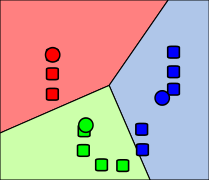
1. 在数据域内（以彩色显示）随机生成k个初始“均值”（在这种情况下，[math]\displaystyle{ k = 3 }[/math]）
2. 通过将每个观察值与最近的平均值相关联来创建k个聚类。此处的分区表示通过该方法生成的Voronoi图。
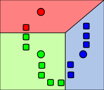
3. [math]\displaystyle{ k }[/math]个簇中每个簇的质心成为新的均值。
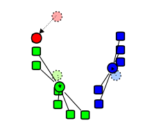
4. 重复步骤2和3，直到达到收敛为止。

该算法不能保证收敛到全局最优，其结果可能取决于初始簇。由于该算法通常速度很快，因此通常会在不同的起始条件下多次运行该算法。然而，最坏情况下的性能可能会很慢：特别是某些点集，甚至在两个维度，会聚指数时间，即 $2 Ω(n)$ 。^[13] 这些点集似乎在实践中似乎没有出现：k-means的平滑运行时间是多项式，这一事实得到了证实。^[14]

“分配”步骤被称为“期望步骤”，而“更新步骤”是最大化步骤，这使得该算法成为广义期望最大化算法的变体。

变体

Jenks自然断点优化：使用单变量数据的k-means。
k-medians clustering使用每个维度中的中位数而不是均值，这样可以最大程度地减少[math]\displaystyle{ L_1 }[/math]规范（出租车的几何形状）。
k-medoids clustering（也称为：围绕中心点的划分 Partitioning Around Medoid,PAM）使用中心点而不是均值，并且这种方式将任意距离函数的距离总和最小化。
模糊C均值聚类 Fuzzy C-Means Clustering是k 均值软聚类版本，其中每个数据点具有属于每个聚类的模糊度。
用期望最大化算法 expectation-maximization algorithm（EM算法）训练的高斯混合模型确保对群集依据概率分配（非确定性分配）和多元高斯分布（非均值）。
k-means++选择初始中心的方式可以为WCSS目标提供可证明的上限。
过滤算法 filtering algorithm使用kd树 kd-trees来提高每个k-means的步长。^[15]
一些方法尝试使用三角形不等式来加快每个k-means步骤。^[16]^[17]^[18]^[19]^[18]^[20]
通过在集群之间交换点来逃避局部最优。^[8]
球形k均值聚类 Spherical k-means clustering算法适用于文本数据。^[21]
分层变体，例如二分k均值 Bisecting k-means，^[22]X均值聚类 X-means clustering^[23]和G均值聚类 G-means clustering^[24] 反复拆分聚类以构建层次结构，还可以尝试自动确定数据集中聚类的最佳数量。
内部集群评估方法（例如集群轮廓）可以帮助确定集群的数量。
Minkowski加权k均值 Minkowski weighted k-means：自动计算聚类特定的特征权重，支持直观的想法，即一个特征在不同的特征上可能具有不同的相关度。^[25]这些权重还可以用于重新缩放给定的数据集，增加了在预期的群集数下优化群集有效性指标的可能性。^[26]
Mini-batch k-means：针对不适合内存的数据集使用“mini batch”样本。^[27]

Hartigan-Wong方法

Hartigan和Wong的方法^[8] 提供了k-means算法的一种变体，它随着不同的解决方案更新而朝着最小平方和问题的局部最小值发展。该方法是一种局部搜索，只要此过程可以改善目标函数，它就会反复尝试将样本重新放置到其他聚类中。如果无法通过改善目标将任何样本重定位到其他群集中，则该方法将停止（以局部最小值计）。以与经典k-means类似的方式，该方法仍然是一种启发式方法，因为它不一定保证最终解是全局最优的。

让[math]\displaystyle{ \varphi(S_j) }[/math]成为[math]\displaystyle{ S_j }[/math]被定义为[math]\displaystyle{ \sum_{x \in S_j} (x - \mu_j)^2 }[/math]，带有[math]\displaystyle{ \mu_j }[/math]集群的中心。

分配： Hartigan-Wong方法开始于将点划分为随机簇[math]\displaystyle{ \{ S_j \}_{j \in \{1, \cdots k\}} }[/math]。

更新：确定[math]\displaystyle{ n,m \in \{1, \ldots, k \} }[/math] and [math]\displaystyle{ x \in S_n }[/math]其以下功能达到最低要求：

[math]\displaystyle{ \Delta(m,n,x) = \varphi(S_n) + \varphi(S_m) - \varphi(S_n \smallsetminus \{ x \} ) - \varphi(S_m \cup \{ x \} ) }[/math]。

为了 [math]\displaystyle{ x,n,m }[/math]达到最低要求 [math]\displaystyle{ x }[/math]从集群中移出[math]\displaystyle{ S_n }[/math]到集群[math]\displaystyle{ S_m }[/math]。

终止：算法终止一次[math]\displaystyle{ \Delta(m,n,x) }[/math]全部大于零[math]\displaystyle{ x,n,m }[/math]。

可以使用不同的移动接受策略。在“ 第一改进”策略中，可以应用任何改进的重定位，而在“ 最佳改进”策略中，所有可能的重定位都经过迭代测试，并且每次迭代仅应用最佳方法。前一种方法有利于速度，而后一种方法是否通常以牺牲额外的计算时间为代价而有利于解决方案质量。[math]\displaystyle{ \Delta }[/math]使用等式也可以有效地计算重定位的结果[37]

[math]\displaystyle{ \Delta(x,n,m) = \frac{ \mid S_n \mid }{ \mid S_n \mid - 1} \cdot \lVert \mu_n - x \rVert^2 - \frac{ \mid S_m \mid }{ \mid S_m \mid + 1} \cdot \lVert \mu_m - x \rVert^2 }[/math]。

k-means算法缺点

在k-means算法中K是事先给定的，这个K值的选定是非常难以估计的。很多时候，事先并不知道给定的数据集应该分成多少个类别才最合适。这也是k-means算法的一个不足。有的算法是通过类的自动合并和分裂，得到较为合理的类型数目K，例如ISODATA算法。关于k-means算法中聚类数目K值的确定在文献中，是根据方差分析理论，应用混合F统计量来确定最佳分类数，并应用了模糊划分熵来验证最佳分类数的正确性。在文献中，使用了一种结合全协方差矩阵的RPCL算法，并逐步删除那些只包含少量训练数据的类。而文献中使用的是一种称为次胜者受罚的竞争学习规则，来自动决定类的适当数目。它的思想是：对每个输入而言，不仅竞争获胜单元的权值被修正以适应输入值，而且对次胜单元采用惩罚的方法使之远离输入值。
在k-means算法中，首先需要根据初始聚类中心来确定一个初始划分，然后对初始划分进行优化。这个初始聚类中心的选择对聚类结果有较大的影响，一旦初始值选择的不好，可能无法得到有效的聚类结果，这也成为k-means算法的一个主要问题。对于该问题的解决，许多算法采用遗传算法（GA），例如文献中采用遗传算法（GA）进行初始化，以内部聚类准则作为评价指标。
从k-means算法框架可以看出，该算法需要不断地进行样本分类调整，不断地计算调整后的新的聚类中心，因此当数据量非常大时，算法的时间开销是非常大的。所以需要对算法的时间复杂度进行分析、改进，提高算法应用范围。在文献中从该算法的时间复杂度进行分析考虑，通过一定的相似性准则来去掉聚类中心的侯选集。而在文献中，使用的k-means算法是对样本数据进行聚类，无论是初始点的选择还是一次迭代完成时对数据的调整，都是建立在随机选取的样本数据的基础之上，这样可以提高算法的收敛速度。

应用

矢量量化

k-means源于信号处理，至今仍在该领域中得到使用。例如，在计算机图形学中，颜色量化是将图像的调色板缩小为固定数量的颜色k的任务。该k-means算法可以很容易地用于此任务，并产生有竞争力的结果。这种方法的一个用例是图像分割。向量量化的其他用途还包括非随机采样，因为k-means可以轻松地用于从大型数据集中选择[math]\displaystyle{ k }[/math]个不同但原型的对象进行进一步分析。

聚类分析

在聚类分析中，可以使用k-means算法将输入数据集划分为[math]\displaystyle{ k }[/math]个分区（集群）。

但是，k-means算法本身不是很灵活，因此用途有限（除了上述矢量量化是k-means算法期望的使用情况）。特别地，当没有外部约束时，已知参数[math]\displaystyle{ k }[/math]难以选择。另一个限制是它不能同其他距离函数或非数值数据一起使用。在此情况下，一些其他的算法更具优势。

特征学习

在（半）监督学习或无监督学习中，k-means聚类被用作特征学习(或字典学习)的一个步骤。^[28]基本方法是：

首先使用输入的训练数据（无需标记）训练k-means聚类表示。然后，将输入投影到新的特征空间中，使用“编码”函数（例如基准与基准位置的基准矩阵乘积）计算质心之间的距离,，或者简单地使用指标函数最近的质心^[28]^[29]或距离的平滑转换。^[30]或者，通过高斯RBF变换样本群集距离，获得径向基函数网络的隐藏层。^[31]

k-means的这种使用已成功地与简单的线性分类器相结合，用于NLP（专门用于命名实体识别）^[32]和计算机视觉中的半监督学习。在用于对象识别时，它可以通过更复杂的特征学习方法（例如自动编码器和受限的Boltzmann机器）表现出可比的性能。^[30]但是，为了达到相同的效果，它通常需要更多的数据支持，因为每个数据点仅有助于一个“功能”。^[28]

示例

使用python的sklearn包实现k-means聚类

本案例中使用k-means方法来对手写阿拉伯数字图像进行分类（分为十类）。

首先是调用一些包

    import time
    import numpy as np
    import pylab as pl
    from sklearn import metrics
    from sklearn.cluster import KMeans
    from sklearn.datasets import load_digits
    from sklearn.decomposition import PCA
    from sklearn.preprocessing import scale

其次要准备数据，这个数据是在sklearn里自带的，是1767个手写数字的图像，每个图像是8*8的矩阵，如下图所示

每个像素都是一个特征，所以原始数据是64个特征。

    
    #-----prepare  data-----------
    np.random.seed(42)
    digits = load_digits()
    data = scale(digits.data)
    n_samples, n_features = data.shape
    n_digits = len(np.unique(digits.target))
    labels = digits.target
    sample_size = 300
    
    print("n_digits: %d, \t n_samples %d, \t n_features %d"
          % (n_digits, n_samples, n_features))
    print(79 * '_')
    print('% 9s' % 'init' ' time  inertia    homo   compl  v-meas     ARI AMI  silhouette')

上述统计量中有些用了简写：

              Shorthand	     full name
                homo	          homogeneity score
                compl	          completeness score
                v-meas	          V measure
                ARI	          adjusted Rand index
                AMI	          adjusted mutual information
                silhouette	  silhouette coefficient

k-means聚类的结果会随着制定类别数和初始点的选择有所不同。我们这里总是聚成十类，因为手写数字一共有十种。至于初始点的选取我们定义三种，k-means++，随机，和PCA降到十个维度后的中心点。

    #---define function and fit data--------------
    def bench_k_means(estimator, name, data):
        t0 = time.clock()
        estimator.fit(data)
        print('% 9s   %.2fs    %i   %.3f   %.3f   %.3f   %.3f   %.3f    %.3f'
              % (name, (time.clock() - t0), estimator.inertia_,
                 metrics.homogeneity_score(labels, estimator.labels_),
                 metrics.completeness_score(labels, estimator.labels_),
                 metrics.v_measure_score(labels, estimator.labels_),
                 metrics.adjusted_rand_score(labels, estimator.labels_),
                 metrics.adjusted_mutual_info_score(labels,  estimator.labels_),
                 metrics.silhouette_score(data, estimator.labels_,
                                          metric='euclidean',
                                          sample_size=sample_size)))
    
    bench_k_means(KMeans(init='k-means++', n_clusters=n_digits, n_init=10),
                  name="k-means++", data=data)
    bench_k_means(KMeans(init='random', n_clusters=n_digits, n_init=10),
                  name="random", data=data)
    # in this case the seeding of the centers is deterministic, hence we run the
    # kmeans algorithm only once with n_init=1
    pca = PCA(n_components=n_digits).fit(data)
    bench_k_means(KMeans(init=pca.components_, n_clusters=n_digits, n_init=1),
                  name="PCA-based",
                  data=data)

上述程序运行完就会出现这样的结果：

       n_digits: 10,          n_samples 1797,         n_features 64
       _______________________________________________________________________________
       init    time  inertia    homo   compl  v-meas     ARI AMI  silhouette
       k-means++   1.40s    69432   0.602   0.650   0.625   0.465   0.598    0.146
          random   1.20s    69694   0.669   0.710   0.689   0.553   0.666    0.147
       PCA-based   0.04s    71820   0.673   0.715   0.693   0.567   0.670    0.150
       _______________________________________________________________________________

我们还可以将原始数据用PCA降到两维，这样所有的数据就可以在二维空间中画出来。然后我们再用降维后的只有两个特征的数据进行k-means分析，聚成十类，然后再画在Voronoi diagram图的背景上。效果如下所示：

聚类效果图

      
    #----Visualize the results on PCA-reduced data------------
    
    reduced_data = PCA(n_components=2).fit_transform(data)
    kmeans = KMeans(init='k-means++', n_clusters=n_digits, n_init=10)
    kmeans.fit(reduced_data)
    # Step size of the mesh. Decrease to increase the quality of the VQ.
    h = .02     # point in the mesh [x_min, m_max]x[y_min, y_max].
    # Plot the decision boundary. For that, we will assign a color to each
    x_min, x_max = reduced_data[:, 0].min() + 1, reduced_data[:, 0].max() - 1
    y_min, y_max = reduced_data[:, 1].min() + 1, reduced_data[:, 1].max() - 1
    xx, yy = np.meshgrid(np.arange(x_min, x_max, h), np.arange(y_min, y_max, h))
    # Obtain labels for each point in mesh. Use last trained model.
    Z = kmeans.predict(np.c_[xx.ravel(), yy.ravel()])
    # Put the result into a color plot
    Z = Z.reshape(xx.shape)
    
    pl.figure(1)
    pl.clf()
    pl.imshow(Z, interpolation='nearest',
              extent=(xx.min(), xx.max(), yy.min(), yy.max()),
              cmap=pl.cm.Paired,
              aspect='auto', origin='lower')
    pl.plot(reduced_data[:, 0], reduced_data[:, 1], 'k.', markersize=2)
    # Plot the centroids as a white X
    centroids = kmeans.cluster_centers_
    pl.scatter(centroids[:, 0], centroids[:, 1],
               marker='x', s=169, linewidths=3,
               color='w', zorder=10)
    pl.title('k-means clustering on the digits dataset (PCA-reduced data)\n'
             'Centroids are marked with white cross')
    pl.xlim(x_min, x_max)
    pl.ylim(y_min, y_max)
    pl.xticks(())
    pl.yticks(())

使用k-means聚类来进行问答类社区的帖子推荐

k-means聚类结果展示

    # -*- coding: utf-8 -*-
    """
    Created on Fri Dec 06 14:15:54 2013
    
    @author: wlf850927
    """
    import os
    import sys
    import scipy as sp
    import numpy as np
    from sklearn.feature_extraction.text import CountVectorizer
    
    vectorizer = CountVectorizer(min_df=1)
    #print(vectorizer) to check all available parameters
    
    
    #----------test sklearn function----------------
    
    content = ["How to format my hard disk", " Hard disk format problems "]
    X = vectorizer.fit_transform(content)
    vectorizer.get_feature_names() 
    print(X.toarray().T)
    
    #----------prepare post data------------------------
    #old posts
    DIR="E:/wulingfei/posts"
    posts = [open(os.path.join(DIR, f)).read() for f in os.listdir(DIR)]
    X_train = vectorizer.fit_transform(posts)
    num_samples, num_features = X_train.shape
    print(vectorizer.get_feature_names())
    #a new post
    new_post = "imaging databases"
    new_post_vec = vectorizer.transform([new_post])
    print(new_post_vec.toarray()) 
    
    #------- calculate raw distances betwee new and old posts and record the shortest one-------------------------
    
    def dist_raw(v1, v2):
        delta = v1-v2
        return sp.linalg.norm(delta.toarray())
    
    best_doc = None
    best_dist = sys.maxint
    best_i = None
    for i in range(0, num_samples):
        post = posts[i]
        if post==new_post:
            continue
        post_vec = X_train.getrow(i)
        d = dist_raw(post_vec, new_post_vec)
        print "=== Post %i with dist = %.2f: %s" % (i, d, post)
        if d<best_dist:
            best_dist = d
            best_i = i
        print("Best post is %i with dist=%.2f" % (best_i, best_dist))
        
    #-------case study: why post 4 and post 5 different ?-----------
    
    print(X_train.getrow(3).toarray())
    print(X_train.getrow(4).toarray())
    
    #conclusion: we should normalize the word count vectors !
    
    #------- calculate new distances betwee new and old posts and record the shortest one----------------
    
    def dist_norm(v1, v2):
        v1_normalized = v1/sp.linalg.norm(v1.toarray())
        v2_normalized = v2/sp.linalg.norm(v2.toarray())
        delta = v1_normalized - v2_normalized
        return sp.linalg.norm(delta.toarray())
        
    best_doc = None
    best_dist = sys.maxint
    best_i = None
    for i in range(0, num_samples):
        post = posts[i]
        if post==new_post:
            continue
        post_vec = X_train.getrow(i)
        d = dist_norm(post_vec, new_post_vec)
        print "=== Post %i with dist = %.2f: %s" % (i, d, post)
        if d<best_dist:
            best_dist = d
            best_i = i
        print("Best post is %i with dist=%.2f" % (best_i, best_dist))
    
    #--Removing less important words (stop words)-------------------
    
    vectorizer = CountVectorizer(min_df=1, stop_words='english')#318 words
    
    sorted(vectorizer.get_stop_words())[0:20]  #show some stop words
      
    X_train = vectorizer.fit_transform(posts)
    num_samples, num_features = X_train.shape
    print(vectorizer.get_feature_names())
    new_post_vec = vectorizer.transform([new_post])
    print(new_post_vec.toarray()) 
        
    best_doc = None
    best_dist = sys.maxint
    best_i = None
    for i in range(0, num_samples):
        post = posts[i]
        if post==new_post:
            continue
        post_vec = X_train.getrow(i)
        d = dist_norm(post_vec, new_post_vec)
        print "=== Post %i with dist = %.2f: %s" % (i, d, post)
        if d<best_dist:
            best_dist = d
            best_i = i
        print("Best post is %i with dist=%.2f" % (best_i, best_dist))
        
        
    #-----------stemming-------------------------
    import nltk.stem 
    english_stemmer = nltk.stem.SnowballStemmer('english')
    english_stemmer.stem("graphics")
    english_stemmer.stem("imaging")
    english_stemmer.stem("buys")
    english_stemmer.stem("buying")
    
    
    class StemmedCountVectorizer(CountVectorizer):
        def build_analyzer(self):
            analyzer = super(StemmedCountVectorizer, self).build_analyzer()
            return lambda doc: (english_stemmer.stem(w) for w in analyzer(doc))
    
    vectorizer = StemmedCountVectorizer(min_df=1, stop_words='english')
    X_train = vectorizer.fit_transform(posts)
    num_samples, num_features = X_train.shape
    new_post_vec = vectorizer.transform([new_post])
        
    best_doc = None
    best_dist = sys.maxint
    best_i = None
    for i in range(0, num_samples):
        post = posts[i]
        if post==new_post:
            continue
        post_vec = X_train.getrow(i)
        d = dist_norm(post_vec, new_post_vec)
        print "=== Post %i with dist = %.2f: %s" % (i, d, post)
        if d<best_dist:
            best_dist = d
            best_i = i
        print("Best post is %i with dist=%.2f" % (best_i, best_dist))
    
    #----------TF-IDF------------------------------------
    
    def tfidf(term, doc, docset):
        tf = float(doc.count(term))/len(doc)
        idf =  np.log(float(len(docset))/(len([doc for doc in docset if term in doc])))
        return tf * idf
    
    a, abb, abc = ["a"], ["a", "b", "b"], ["a", "b", "c"]
    
    D = [a, abb, abc]
    
    
    print(tfidf("a", abc, D))
    print(tfidf("b", abc, D))
    print(tfidf("c", abc, D))
    
    from sklearn.feature_extraction.text import TfidfVectorizer
    class StemmedTfidfVectorizer(TfidfVectorizer):
        def build_analyzer(self):
            analyzer = super(TfidfVectorizer,self).build_analyzer()
            return lambda doc: (english_stemmer.stem(w) for w in analyzer(doc))
    
    
    vectorizer = StemmedTfidfVectorizer(min_df=1,stop_words='english', decode_error='ignore')
    X_train = vectorizer.fit_transform(posts)
    num_samples, num_features = X_train.shape
    new_post_vec = vectorizer.transform([new_post])
    print(vectorizer.get_feature_names())
    print(new_post_vec.toarray()) 
    
    best_doc = None
    best_dist = sys.maxint
    best_i = None
    for i in range(0, num_samples):
        post = posts[i]
        if post==new_post:
            continue
        post_vec = X_train.getrow(i)
        d = dist_norm(post_vec, new_post_vec)
        print "=== Post %i with dist = %.2f: %s" % (i, d, post)
        if d<best_dist:
            best_dist = d
            best_i = i
        print("Best post is %i with dist=%.2f" % (best_i, best_dist))
    
    #------summary of data clean (how to illuminate noise)------------
    '''
    1. Tokenize (cut text into words)
    2. Stemming (clean the form of words)
    3. Throw away words that accur too often (stop_words='english')
    4. Throw away words that accur so seldom (min_df=1) 
    5. Use the index of TF - IDF
    '''
    #--------clustering posts using K means-----------------
    '''
    1. flat clustering : you need to set the number of clusters
    2. hierarchical clustering : you need to balance between H (level of hierarchy) and N (number 
    of clusters)
    '''
    
    import sklearn.datasets
    MLCOMP_DIR = r"E:/wulingfei/20news_18828"
    '''
    data = sklearn.datasets.load_mlcomp("20news-18828",set_='raw', mlcomp_root=MLCOMP_DIR)
    print(data.filenames)
    print(len(data.filenames))
    data.target_names
    train_data = sklearn.datasets.load_mlcomp("20news-18828", "train",mlcomp_root=MLCOMP_DIR)
    print(len(train_data.filenames))
    test_data = sklearn.datasets.load_mlcomp("20news-18828", "test", mlcomp_root=MLCOMP_DIR)
    print(len(test_data.filenames))
    '''
    
    groups = ['comp.graphics', 'comp.os.ms-windows.misc', 'comp.sys. \
    ibm.pc.hardware', 'comp.sys.ma c.hardware', 'comp.windows.x', 'sci. \
    space']
    train_data = sklearn.datasets.load_mlcomp("20news-18828", "train", 
                                              mlcomp_root=MLCOMP_DIR, categories=groups)
    print(len(train_data.filenames))
    
    
    vectorizer = StemmedTfidfVectorizer(min_df=10, max_df=0.5, 
                                        stop_words='english', decode_error='ignore')
                                        
    vectorized = vectorizer.fit_transform(train_data.data)
    num_samples, num_features = vectorized.shape
    num_clusters = 50
    from sklearn.cluster import KMeans
    km = KMeans(n_clusters=num_clusters, init='random', n_init=1, verbose=1)
    km.fit(vectorized)
    km.labels_
    len(km.labels_)
    km.cluster_centers_.shape
    
    new_post='''
    Disk drive problems. Hi, I have a problem with my hard disk. 
    After 1 year it is working only sporadically now. 
    I tried to format it, but now it doesn't boot any more. 
    Any ideas? Thanks.
    '''
    
    new_post_vec = vectorizer.transform([new_post])
    new_post_label = km.predict(new_post_vec)[0]
    similar_indices = (km.labels_==new_post_label).nonzero()[0]
    similar = []
    for i in similar_indices:
        dist = sp.linalg.norm((new_post_vec - vectorized[i]).toarray())
        similar.append((dist, train_data.data[i]))
    
    similar = sorted(similar)
    
    print(len(similar))
    
    
    
    show_at_1 = similar[0]
    show_at_2 = similar[int(len(similar)/2)]
    show_at_3 = similar[-1]

data 把这段话变成五句，存成五个txt文件，放到“post”文件里，就是示例数据：

['This is a toy post about machine learning. Actually, it contains\nnot much interesting stuff.', 'Imaging databases can get huge.', 'Most imaging databases safe images permanently.', 'Imaging databases store images.', 'Imaging databases store images. Imaging databases store\nimages. Imaging databases store images.']

开源软件包/代码

Orange

k-means常用免费/开源代码如下：

Accord.NET：含有C＃实现的用于k-means，k-means++和K-modes。
ALGLIB：包含针对k-means和k-means++的并行C++和C＃实现。
AOSP：包含用于k-means 的Java实现。
CrimeStat：实现了两种空间k 均值算法，其中一种允许用户定义起始位置。
ELKI：包含k-means（具有Lloyd和MacQueen迭代，以及不同的初始化，例如k-means++初始化）和各种更高级的聚类算法。
Julia：在JuliaStats Clustering包中包含一个k-means实现。
KNIME：包含节点k-means和K-medoids。
Mahout：包含基于MapReduce的k-means。

Weka

mlpack：包含k-means的C++实现。
Octave：包含k-means。
OpenCV：包含一个k-means实现。
Orange：包含用于k-均值聚类的组件，可自动选择k和聚类轮廓评分。
PSPP：包含k-means，QUICK CLUSTER命令对数据集执行k-means聚类。
R：包含三个k-means变体。
SciPy和scikit-learn：包含多个k-means实现。
Spark MLlib：实现了分布式k-means 算法。
Torch：包含一个unsup软件包提供k-means聚类。
Weka：包含k-means和x-means。

参考文献

↑ MacQueen, J. B., Retrieved (1967) Some Methods for classification and Analysis of Multivariate Observations.Proceedings of 5th Berkeley Symposium on Mathematical Statistics and Probability..1.(281--297)
↑ Steinhaus, Hugo (1957) "Sur la division des corps matériels en parties".Bull. Acad. Polon. Sci. (in French).3.4:(801--804)
↑ Lloyd, Stuart P., Stuart P., Retrieved (1982) Least square quantization in PCM", "Least squares quantization in PCM.IEEE Transactions on Information Theory.28.2:(129--137)
↑ Forgy, Edward W. (1965) "Cluster analysis of multivariate data: efficiency versus interpretability of classifications".Biometrics.21.(768--769)
↑ Pelleg, Dan; Moore, Andrew (1999). "Accelerating exact k -means algorithms with geometric reasoning". Proceedings of the Fifth ACM SIGKDD International Conference on Knowledge Discovery and Data Mining - KDD '99 (in English). San Diego, California, United States: ACM Press: 277–281. doi:10.1145/312129.312248. ISBN 9781581131437.
↑ MacKay, David (2003). "Chapter 20. An Example Inference Task: Clustering". Information Theory, Inference and Learning Algorithms. Cambridge University Press. pp. 284–292. ISBN 978-0-521-64298-9. http://www.inference.phy.cam.ac.uk/mackay/itprnn/ps/284.292.pdf.
↑ Since the square root is a monotone function, this also is the minimum Euclidean distance assignment.
↑ ^8.0 ^8.1 ^8.2 Hartigan, J. A.; Wong, M. A. (1979). "Algorithm AS 136: A k-Means Clustering Algorithm". Journal of the Royal Statistical Society, Series C. 28 (1): 100–108. JSTOR 2346830.
↑ ^9.0 ^9.1 Hamerly, Greg; Elkan, Charles (2002). Alternatives to the k-means algorithm that find better clusterings (PDF). {{cite conference}}: Unknown parameter |booktitle= ignored (help)
↑ Celebi, M. E.; Kingravi, H. A.; Vela, P. A. (2013). "A comparative study of efficient initialization methods for the k-means clustering algorithm". Expert Systems with Applications. 40 (1): 200–210. arXiv:1209.1960. doi:10.1016/j.eswa.2012.07.021.
↑ Bradley, Paul S.; Fayyad, Usama M. (1998). "Refining Initial Points for k-Means Clustering". Proceedings of the Fifteenth International Conference on Machine Learning.
↑ Bradley, Paul S.; Fayyad, Usama M. (1998). "Refining Initial Points for k-Means Clustering". Proceedings of the Fifteenth International Conference on Machine Learning.
↑ Vattani, A. (2011). "k-means requires exponentially many iterations even in the plane" (PDF). Discrete and Computational Geometry. 45 (4): 596–616. doi:10.1007/s00454-011-9340-1.
↑ Arthur, David; Manthey, B.; Roeglin, H. (2009). k-means has polynomial smoothed complexity. arXiv:0904.1113. {{cite conference}}: Unknown parameter |booktitle= ignored (help)
↑ Kanungo, Tapas; Mount, David M.; Netanyahu, Nathan S.; Piatko, Christine D.; Silverman, Ruth; Wu, Angela Y. (2002). "An efficient k-means clustering algorithm: Analysis and implementation" (PDF). IEEE Transactions on Pattern Analysis and Machine Intelligence. 24 (7): 881–892. doi:10.1109/TPAMI.2002.1017616. Retrieved 2009-04-24.
↑ Phillips, Steven J. (2002-01-04). "Acceleration of K-Means and Related Clustering Algorithms". In Mount, David M.. Acceleration of k-Means and Related Clustering Algorithms. Lecture Notes in Computer Science. 2409. Springer Berlin Heidelberg. pp. 166–177. doi:10.1007/3-540-45643-0_13. ISBN 978-3-540-43977-6.
↑ Elkan, Charles (2003). Using the triangle inequality to accelerate k-means (PDF). {{cite conference}}: Unknown parameter |booktitle= ignored (help)
↑ ^18.0 ^18.1 Hamerly, Greg. "Making k-means even faster". CiteSeerX 10.1.1.187.3017. {{cite journal}}: Cite journal requires |journal= (help)
↑ Hamerly, Greg; Drake, Jonathan (2015). Accelerating Lloyd's algorithm for k-means clustering. pp. 41–78. doi:10.1007/978-3-319-09259-1_2. ISBN 978-3-319-09258-4.
↑ Drake, Jonathan (2012). "Accelerated k-means with adaptive distance bounds" (PDF). The 5th NIPS Workshop on Optimization for Machine Learning, OPT2012.
↑ Dhillon, I. S.; Modha, D. M. (2001). "Concept decompositions for large sparse text data using clustering". Machine Learning. 42 (1): 143–175. doi:10.1023/a:1007612920971.
↑ Steinbach, M.; Karypis, G.; Kumar, V. (2000). ""A comparison of document clustering techniques". In". KDD Workshop on Text Mining. 400 (1): 525–526.
↑ Pelleg, D.; & Moore, A. W. (2000, June). "X-means: Extending k-means with Efficient Estimation of the Number of Clusters". In ICML, Vol. 1
↑ Hamerly, Greg; Elkan, Charles (2004). Advances in Neural Information Processing Systems. 16: 281. {{cite journal}}: Missing or empty |title= (help)
↑ Amorim, R. C.; Mirkin, B. (2012). "Minkowski Metric, Feature Weighting and Anomalous Cluster Initialisation in k-Means Clustering". Pattern Recognition. 45 (3): 1061–1075. doi:10.1016/j.patcog.2011.08.012.
↑ Amorim, R. C.; Hennig, C. (2015). "Recovering the number of clusters in data sets with noise features using feature rescaling factors". Information Sciences. 324: 126–145. arXiv:1602.06989. doi:10.1016/j.ins.2015.06.039.
↑ Sculley, David (2010). Web-scale k-means clustering. ACM. pp. 1177–1178. Retrieved 2016-12-21. {{cite conference}}: Unknown parameter |booktitle= ignored (help)
↑ ^28.0 ^28.1 ^28.2 Coates, Adam; Ng, Andrew Y. (2012). "Learning feature representations with k-means" (PDF). Neural Networks: Tricks of the Trade. Springer. {{cite encyclopedia}}: Unknown parameter |editors= ignored (help)
↑ Csurka, Gabriella; Dance, Christopher C.; Fan, Lixin; Willamowski, Jutta; Bray, Cédric (2004). Visual categorization with bags of keypoints (PDF). ECCV Workshop on Statistical Learning in Computer Vision.
↑ ^30.0 ^30.1 Coates, Adam; Lee, Honglak; Ng, Andrew Y. (2011). An analysis of single-layer networks in unsupervised feature learning (PDF). International Conference on Artificial Intelligence and Statistics (AISTATS). Archived from the original (PDF) on 2013-05-10.
↑ Schwenker, Friedhelm; Kestler, Hans A.; Palm, Günther (2001). "Three learning phases for radial-basis-function networks". Neural Networks. 14 (4–5): 439–458. CiteSeerX 10.1.1.109.312. doi:10.1016/s0893-6080(01)00027-2. PMID 11411631.
↑ Lin, Dekang; Wu, Xiaoyun (2009). Phrase clustering for discriminative learning (PDF). Annual Meeting of the ACL and IJCNLP. pp. 1030–1038.

编者推荐

数据科学家需要了解的5种聚类算法