人工神经网络

人工神经网络 (ANNs) 或 联结主义 系统 或许是受到构成动物大脑的生物神经网络启发的计算系统[1]。这种系统通过分析样本“学习”执行任务,通常不需要用任何具体的任务规则编程。例如,在图像识别,他们可能通过分析被手动标记成“有猫”和“无猫”的示例图像来学习识别包含猫的图像并利用结果识别其他图像中的猫。他们不需要任何关于猫的先验知识以完成这个任务,例如它们有毛,尾巴,胡须和猫科动物的脸。它们自动地从它们处理的学习材料中产生识别特征。
人工神经网络是基于一些称为人工神经元的相连单元或节点,它们宽泛地模拟了一个生物的大脑中的神经元。每个连接好像一个生物的大脑中的突触,它们可以将信号从一个人工神经元传递到另一个。一个接收信号的人工神经元可以处理它然后发信号给它连接到的额外的人工神经元。
在通常的人工神经网络实现中,在人工神经元之间连接的信号是一个实数,每个人工神经元的输出则由它输入之和的某个非线性函数计算。人工神经元之间的连接成为“边”。人工神经元和边通常有一个随学习进行而调整的权重。这个权重增加或减少一个连接处的信号强度。人工神经元可能有一个阈值以便信号只有在聚集的信号越过这个阈值时才发出。一般地,人工神经元聚集成层,不同的层可能对它们的输入执行不同种类的转换。信号从第一层(输入层)传递到最后一层(输出层),可能会多次穿过这些层。
人工神经网络起初希望达到的目标是用人脑相同方式解决问题。然而,随着时间的发展,人们将注意力转向执行具体的任务,导致了人工神经网络的发展从生物学的偏离。人工神经网络被用于多种任务,包括计算机视觉,语音识别,机器翻译,社交网络滤波,棋类和电子游戏和医疗诊断。
历史
Warren McCulloch 和 Walter Pitts[2] 构造了一个关于基于数学和算法的神经网络计算模型,称为阈值逻辑。这个模型为神经网络研究铺平了两条道路。一个关注大脑中的生物学过程,而另一个关注神经网络向人工智能的应用。这个工作引领了神经网络的工作以及他们与有限状态机(Finite state machine)的联系[3]。
赫布学习(Hebbian learning)
在19世纪40年代晚期,D.O.Hebb[4] 基于神经可塑性的机制构造了一个学习假设,被称为赫布学习。赫布学习是无监督学习(unsupervised learning)。这形成了长程增强效应模型。在1948年,研究者开始将这些想法和B类图灵机应用到计算模型上。
Farley 和Clark[5] 首先使用计算机器,后来称作“计算器”,来模拟赫布网络。其他神经网络计算机器被RochesterHolland, Habit 和 Duda创造[6].
Rosenblatt[7] 创造了感知机,这是一种模式识别算法。Rosenblatt 使用数学记号描述了无法用基本感知机识别的逻辑电路,如那时无法被神经网络处理的异或电路[8] 。
1959年,Nobel laureateHubel和Wiesel在初级视皮层发现了两种类型的细胞:简单细胞(simple cell)和复杂细胞(complex cell)[9],并基于他们的发现提出了一个生物学模型,
第一个有多层的功能网络由Ivakhnenko和Lapa在1965年发表,它成为了数据处理的组方法[10][11][12]
在发现了两个执行神经网络的计算机器关键问题的Minsky和Papert[13] 研究的[1]后,神经网络的研究停滞了。第一个是基本感知机不能处理异或电路。第二个是计算机没有足够的处理能力来有效地处理大型神经网络需要的任务。神经网络研究步伐放缓直到计算机具有了更好的运算能力。
更多的人工智能专注于算法执行的高层面(符号的)模型,以知识体现在如果-那么规则中的专家系统为特征。直到19世纪80年代末期,研究扩展到低层面(次符号的)[2],以知识体现在一个认知模型的参数中为特征。
反向传播(Backpropagation)
Werbos的反向传播算法重新燃起了人们对于神经网络和学习的兴趣,它有效地解决了异或问题并且更普遍地加速了多层网络的训练。反向传播通过修改每个节点的权重,反向分散了贯穿每个层中的梯度[8] 。
在19世纪80年代中期,并行分布处理以联结主义的名义变得受欢迎,Rumelhart和McClelland描述了联结主义模拟神经过程的作用。[14]
支持向量机(Support vector machine)和其他更简单的方法如线性分类器在机器学习中的受欢迎程度逐步超过了神经网络。然而,使用神经网络改变了一些领域,例如蛋白质结构的预测。[15][16]
1992年最大池化被引入帮助最小转移不变性和最大容忍性来变形,有助于3D物体识别。[17][18][19]
2010年,通过最大池化训练的反向传播训练被GPU加速,显示出超过其他池化变体的性能。[20]
梯度消失问题影响使用反向传播的多层[前馈神经网络https://en.wikipedia.org/wiki/Feedforward_neural_network 前馈神经网络] 和循环神经网络(RNN)。[21][22] 由于梯度从一层到另一层传播,它们随着层数指数级减小,这样阻碍了依赖这些误差的的神经元权重的调整,尤其影响深度网络。
为了解决这个问题,Schmidhuber采用了一种多层网络结构,通过无监督学习每次预训练一级然后使用反向传播很好地调整[23]。例如,Behnke 在图像重建和人脸定位中只依赖梯度符号。[24]
Hinton提出了使用连续层的二进制或潜变量实数受限玻尔兹曼机[25]来模拟每一层学习一种高级别表征。一旦很多层被充分学习,这种深度结构可能像生成模型一样被使用,通过在下采样(一个古老的方法)模型时从顶层特征激活处复制数据。[26][27] 2012年Ng 和Dean创造了一个只通过看YouTube视频中未标记的图像学习识别例如猫这样更高层概念的网络。[28]
在训练深度神经网络中早期的挑战被成功地用无监督预训练等方法处理,与此同时可见的计算性能通过GPU和分布计算的使用提升。神经网络被部署在大规模,尤其是在图像和视觉识别问题上。这被称为“深度学习”
基于硬件的设计(Hardware-based designs)
用于生物学模拟和神经形态计算的计算设备[29]在CMOS创建。用于很大规模主成分分析和卷积的纳米元件可能创造一类新的神经计算,因为它们根本上是模拟的而不是数字的(尽管第一个实现使用数字设备)[30]。在Schmidhuber 组的.Ciresan 和 colleagues[31]表明,尽管有梯度消失问题,GPU使反向传播对多层前馈神经网络更可行。
竞赛
在2009~2012年间,循环神经网络和Schmidhuber的研究组发展的深度前馈神经网络赢得了八个在模式识别和[3][32][33]的国际竞赛。例如,Graves的双向和多维长短期记忆(LSTM)[34][35][36][37]在2009文件分析和识别国际会议上的连笔手写识别中赢得了三个比赛,而没有任何关于要学习的那三种语言的先验知识。[36][35]
Ciresan 和同事赢得了模式识别比赛,包括IJCNN2011交通信号识别比赛[38],ISBI2012叠加电子显微镜中的神经结构分割挑战[39]和其他比赛。他们的神经网络是第一个在基准测试数据集中达到能挑战甚至超过人类表现[40]的模式识别模型。这些基准数据集例如交通信号识别(ijcnn2012)或者MNIST手写数字问题
研究人员演示了深度神经网络接口下的隐式马尔科夫模型,它依赖上下文定义神经网络输出层的状态,可以降低在大量词汇语音识别——例如语音搜索——中的误差。【?】
这种方法基于GPU的实现[41]赢得了很多模式识别竞赛,包括IJCNN2011交通信号识别比赛[38],ISBI2012叠加电子显微镜中的神经结构分割挑战[39]和ImageNet竞赛[42] 以及其他比赛。
被简单和复杂细胞启发的,与新认知机[43] 相似的深度的高度非线性神经结构和“标准视觉结构”[44],被Hinton提出的无监督方法预训练[45][26]。他实验室的一个团队赢得了一个2012年的竞赛,这个竞赛由Merck资助来设计可以帮助找到能识别新药物分子的软件。[46]
卷积网络(Convolutional networks)
自2011起,深度学习前馈网络的艺术状态在卷积层和最大池化层[41][47]之间切换,位于几层全连接或稀疏连接层和一层最终分类层之上。学习通常不需要非监督预学习。
这种监督深度学习方法第一次达到在某些任务中能挑战人类表现的水平。[40]
ANN能够保证平移不变形来处理在大型聚类场景中的小和大的自然物体,仅当不变性扩展超过平移,对于所有ANN学习的概念如位置,类型(物体分类标记),大小,亮度等。 这被称为启发式网络 (DNs)[48] 具体实现有哪里-什么网络(Where-What Networks), WWN-1 (2008)[49]到 WWN-7 (2013).[50]
模型
一个“人工神经网络”是一个称为人工神经元的简单元素的网络,它们接收输入,根据输入改变内部状态(“激活”),然后依靠输入和激活产生输出,通过连接某些神经元的输出到其他神经元的输入的“网络”形式构成了一个有向的有权图。权重和计算激活的函数可以被称为“学习”的过程改变,这被学习规则控制。[51]
人工神经网络的组成部分(Components of an artificial neural network)
神经元(Neurons)
一个有标记[math]\displaystyle{ {j} }[/math] 的神经元从上一层神经元接收输入 [math]\displaystyle{ {p_j}(t) }[/math] ,这些上一层由下面的部分组成:[51]
- 一个激活 [math]\displaystyle{ {{a_j}(t)} }[/math], 取决于一个离散时间参数,
- 可能有一个阈值 [math]\displaystyle{ \theta_j }[/math], 保持不变除非被学习函数改变,
- 一个激活函数 [math]\displaystyle{ f }[/math] ,从 [math]\displaystyle{ {{a_j}(t)} }[/math], [math]\displaystyle{ \theta_j }[/math]和网络输入[math]\displaystyle{ {p_j}(t) }[/math] 计算在给定时间[math]\displaystyle{ {t+1} }[/math]新的激活
- [math]\displaystyle{ {a_j}(t+1) = f({a_j}(t), {p_j}(t), \theta_j) }[/math],
- 和一个 输出函数 [math]\displaystyle{ f_{out} }[/math] 计算从激活函数得到的输出
- [math]\displaystyle{ {o_j}(t) = f_{out}({a_j}(t)) }[/math].
通常输出函数只是简单的恒等函数
一个“输入神经元”没有上一层网络,但作为整个网络的输入接口。同样地,一个“输出神经元”没有下一层而作为整个网络的输出接口。
连接和权重(Connections and weights)
网络由连接组成,每个连接传递一个神经元的输出 [math]\displaystyle{ {i} }[/math] 到一个神经元的输入 [math]\displaystyle{ {j} }[/math]. 从这个角度来说, [math]\displaystyle{ {i} }[/math] 是 [math]\displaystyle{ {j} }[/math] 的前驱, [math]\displaystyle{ {j} }[/math] 是 [math]\displaystyle{ {i} }[/math] 的后继.每个连接被赋予一个权重 [math]\displaystyle{ {w_{ij}} }[/math].[51]有时一个偏置项加在输入的总权重和上,用作变化激活函数的阈值。[52].
传播函数(Propagation function)
“传播函数”计算“从前驱神经元的输出[math]\displaystyle{ o_i(t) }[/math]到神经元 [math]\displaystyle{ {j} }[/math]的输入”[math]\displaystyle{ p_j(t) }[/math]通常有这种形式:[51]
- [math]\displaystyle{ {p_j}(t) = {\sum_{i}} {o_i}(t) {w_{ij}} }[/math]
当偏置值加在函数上时,上面的形式变成下面的:[53]
- [math]\displaystyle{ {p_j}(t) = {\sum_{i}} {o_i}(t) {w_{ij}}+ {w_{0j}} }[/math],
其中[math]\displaystyle{ {{w_{0j}}} }[/math]是偏置。
学习规则(Learning rule)
“学习规则”是一个改变神经网络参数的规则或算法,以便于对网络给定的输入产生偏好的输出。这个学习过程 改变网络中的变量权重和阈值。[51]
作为函数的神经网络(Neural networks as functions)
神经网络模型可以被看成简单的数学模型,定义为一个函数[math]\displaystyle{ \textstyle f : X \rightarrow Y }[/math] 或者是一个 [math]\displaystyle{ \textstyle X }[/math] 上或 [math]\displaystyle{ \textstyle X }[/math] 和[math]\displaystyle{ \textstyle Y }[/math]上的分布。有时模型与一个特定学习规则紧密联系。短语“ANN模型”的通常使用确实是这种函数的“类”的定义(类的成员被不同参数,连接权重或结构的细节如神经元数量或他们的连接获得) 数学上,一个神经元的网络函数 [math]\displaystyle{ \textstyle f(x) }[/math] 被定义为其他函数[math]\displaystyle{ {{g_i}(x)} }[/math]的组合,它可以之后被分解为其他函数。这可以被方便地用一个网络结构表示,它有箭头描述函数间的依赖关系。一类广泛应用的组合是“非线性加权和”, [math]\displaystyle{ \textstyle f(x) = K \left(\sum_i w_i g_i(x)\right) }[/math], 其中 [math]\displaystyle{ \textstyle K }[/math] (通常称为激活函数[54]) 是某种预定义的函数,如双曲正切或双弯曲函数 或柔性最大值传输函数或线性整流函数。激活函数最重要的特点是它随输入值变化提供一个平滑的过渡,例如,在输入中一个小的变化产生输出中一个小的变化 。下面指的是一组函数 [math]\displaystyle{ \textstyle g_i }[/math]作为向量 [math]\displaystyle{ \textstyle g = (g_1, g_2, \ldots, g_n) }[/math].
.svg.png)
本图描述了 [math]\displaystyle{ {f} }[/math]的带有箭头指示出的变量间依赖的这样一种分解,这些可以用两种方式解释。 第一种视角是功能上的:输入[math]\displaystyle{ \textstyle x }[/math] 转化成一个三维向量[math]\displaystyle{ \textstyle h }[/math], 它接着转化为一个二维向量 [math]\displaystyle{ \textstyle g }[/math],它最终转化成 [math]\displaystyle{ {f} }[/math]. 这种视角在优化中经常遇到。 第二种视角是概率上的:随机变量 [math]\displaystyle{ {F = f(G)} }[/math]取决于随机变量 [math]\displaystyle{ \textstyle G = g(H) }[/math],它取决于 [math]\displaystyle{ \textstyle H=h(X) }[/math], 它取决于随机变量 [math]\displaystyle{ \textstyle X }[/math].。这种视角在图模型中经常遇到。 这两种视角大部分等价。不论哪种情况,对于这种特定的结构,单独层的组成互相独立(例如,[math]\displaystyle{ \textstyle g }[/math] 的组成,给定它们的输入[math]\displaystyle{ \textstyle h }[/math]互相独立) 这自然地使实现中的并行成为可能。
 前述的网络通常称为前馈神经网络,因为它们的图是有向无环图。带有环的网络通常称为循环神经网络。这种网络通常被图片顶部的方式描述,其中 [math]\displaystyle{ {f} }[/math] 依赖它自己,而一个隐含的时间依赖没有显示。
学习
神经网络的学习能力吸引了人们最多的兴趣。给定一个特定的“任务”和一类函数[math]\displaystyle{ \textstyle F }[/math]待解决,学习意味着使用一组观测值寻找[math]\displaystyle{ {f^{*}} \in F }[/math],它以某种最优的道理解决任务。 这引发了定义一个损失函数 [math]\displaystyle{ {C} : {F} \rightarrow {\mathbb{R}} }[/math]使得对于最优解[math]\displaystyle{ {f^{*}} }[/math],[math]\displaystyle{ {C}(f^{*}) \leq C(f) }[/math][math]\displaystyle{ \forall {f} \in {F} }[/math]—— 也就是没有解有比最优解更小的损失。 损失函数[math]\displaystyle{ {C} }[/math]是学习中一个重要的概念,因为它是衡量一个特定的解距离一个解决问题的最优解有多远。学习算法搜索解空间寻找一个有最小可能损失的函数。
对于解依赖数据的应用,损失必须必要地作为观测值的函数,否则模型会数据无关。通常定义为一个只能近似的统计量。一个简单的例子是考虑找到最小化[math]\displaystyle{ {C}=E\left[(f(x) - y)^2\right] }[/math]的模型 [math]\displaystyle{ {f} }[/math],对于数据对[math]\displaystyle{ \textstyle (x,y) }[/math] 来自分布[math]\displaystyle{ \textstyle \mathcal{D} }[/math].。在实际情况下我们可能只有 [math]\displaystyle{ \textstyle N }[/math]从 [math]\displaystyle{ \textstyle \mathcal{D} }[/math]采样,这样,对于上面的例子我们只能最小化 [math]\displaystyle{ \textstyle \hat{C}=\frac{1}{N}\sum_{i=1}^N (f(x_i)-y_i)^2 }[/math]. 因此,损失被在数据的一个样本上而不是在整个分布上最小化。
当 [math]\displaystyle{ \textstyle N \rightarrow \infty }[/math],必须使用在线机器学习的某种形式 ,其中损失随着每次观测到新的样本而减小。尽管通常当[math]\displaystyle{ \textstyle \mathcal{D} }[/math]固定时使用在线机器学习,它在分布随时间缓慢变化时最有用。在神经网络方法中,一些种类的在线机器学习通常被用于无限数据集。
选择一个损失函数
虽然可能定义一个专用的损失函数,通常使用一个特定的损失函数,无论因为它有需要的性质(例如凸性质)或因为它从问题的一种特定公式中自然产生(例如在概率公式中模型的后验概率可以被用作相反损失)。最后,损失函数取决于任务。
反向传播
一个深度神经网络可以使用标准反向传播算法判别地训练。反向传播是一种计算关于ANN中权重的损失函数(产生与给定状态相联系的损失)梯度的方法。
连续反向传播的基础[10][55][56][57] 由Kelley[58] 在1960和Bryson在1961[59]使用动态编程的原则从控制论引出。1962,Dreyfus发表了只基于链式法则[60]的更简单的衍生。1969,Bryson和Ho把它描述成一种多级动态系统优化方法。[61][62]1970,Linnainmaa最终发表了嵌套可微函数[63][64] 的离散连接网络自动差分机(AD)的通用方法。这对应于反向传播的现代版本,它在网络稀疏时仍有效[10][55][65][66]。1973[67] ,Dreyfus使用反向传播适配与误差梯度成比例的控制器参数。1974,Werbos提出将这个规则应用到ANN上的可能[68],1982他将LInnainmaa的AD方法以今天广泛使用的方式应用到神经网络上[55][69]。1986, Rumelhart, Hinton和Williams注意到这种方法可以产生有用的神经网络隐藏层到来数据的内部表征。[70] 1933,Wan第一个[10] 用反向传播赢得国际模式识别竞赛。[71]
反向传播的权重更新可以通过随机梯度下降完成,使用下面的等式:
- [math]\displaystyle{ w_{ij}(t + 1) = w_{ij}(t) + \eta\frac{\partial C}{\partial w_{ij}} +\xi(t) }[/math]
其中[math]\displaystyle{ \eta }[/math] 是学习速率, [math]\displaystyle{ {C} }[/math]是损失函数, [math]\displaystyle{ \xi(t) }[/math] 是一个随机项。损失函数的选择由如学习类型(监督,无监督,强化等等)和激活函数等因素决定。例如,当在多类分类问题上使用监督学习,激活函数和损失函数的通常选择分别是柔性最大值传输函数和交叉熵函数。柔性最大值传输函数定义为 [math]\displaystyle{ p_j = \frac{\exp(x_j)}{\sum_k \exp(x_k)} }[/math] 其中 [math]\displaystyle{ p_j }[/math] 代表类的概率(单元[math]\displaystyle{ {j} }[/math]的输出), [math]\displaystyle{ x_j }[/math] 和 [math]\displaystyle{ x_k }[/math] 分别代表单元[math]\displaystyle{ {j} }[/math]和[math]\displaystyle{ k }[/math]在相同程度上的总输入。交叉熵定义为 [math]\displaystyle{ {C} = -\sum_j d_j \log(p_j) }[/math] 其中 [math]\displaystyle{ d_j }[/math] 代表输出单元[math]\displaystyle{ {j} }[/math] 的目标概率, [math]\displaystyle{ p_j }[/math] 是应用激活函数后 [math]\displaystyle{ {j} }[/math]的输出概率。[72]
这可以被用于以二元掩码的形式输出目标包围盒。它们也可以用于多元回归来增加局部精度。基于DNN的回归除作为一个好的分类器外还可以学习捕获几何信息特征。它们免除了显式模型部分和它们的关系。这有助于扩大可以被学习的目标种类。模型由多层组成,每层有一个线性整流单元作为它的非线性变换激活函数。一些层是卷积的,其他层是全连接的。每个卷积层有一个额外的最大池化。这个网络被训练最小化L2 误差 来预测整个训练集范围的掩码包含代表掩码的包围盒。【?】
反向传播的替代包括极端学习机[73],不使用回溯法[74]训练的“无权重”[75][76]网络[77],和非联结主义神经网络
学习范式(Learning paradigms)
三种主要学习范式对应于特定学习任务。它们是:监督学习,无监督学习和强化学习
监督学习(Supervised learning)
监督学习使用一组例子对[math]\displaystyle{ {(x, y)}, {x \in X}, {y \in Y} }[/math],目标是在允许的函数类中找到一个函数 [math]\displaystyle{ f : X \rightarrow Y }[/math] 匹配例子。 换言之,我们希望推断数据隐含的映射;损失函数与我们的映射和数据间的不匹配相关,它隐含了关于问题域的先验知识。[78]
通常使用的损失函数是均方误差,它对所有的例子对在网络输出 [math]\displaystyle{ f(x) }[/math]和目标值[math]\displaystyle{ y }[/math]之间最小化平均平方误差。最小化损失对一类叫做多层感知机(MLP)的一类神经网络使用了梯度下降,产生了训练神经网络的反向传播算法。 监督学习范式中的任务是模式识别(也被称为分类)和回归(也被称为函数逼近)。监督学习范式也可适用于序列数据(例如手写,语音和手势识别)。这可以被认为是和“老师”学习,以一个根据迄今为止得到解的质量提供连续反馈的函数形式。
无监督学习(Unsupervised learning)
在无监督学习中,给定一些数据 [math]\displaystyle{ \textstyle x }[/math] ,要最小化损失函数 ,损失函数可以是数据[math]\displaystyle{ \textstyle x }[/math]和网络输出[math]\displaystyle{ {f} }[/math]的任何函数。 损失函数依赖任务(模型的域)和任何先验的假设(模型的隐含性质,它的参数和观测值) 一个琐碎的例子是,考虑模型[math]\displaystyle{ {{f(x)}={a}} }[/math]其中 [math]\displaystyle{ \textstyle a }[/math] 是一个常数,损失函数为 [math]\displaystyle{ \textstyle C=E[(x - f(x))^2] }[/math]. 最小化这个损失产生了一个 [math]\displaystyle{ \textstyle a }[/math] 的值,它与数据均值相等。损失函数可以更加复杂。它的形式取决于应用:举个例子,在压缩中它可以与[math]\displaystyle{ \textstyle x }[/math] 和 [math]\displaystyle{ \textstyle f(x) }[/math]间的交互信息有关,在统计建模中,它可以与模型给出数据的后验概率有关。(注意在这两个例子中这些量应当被最大化而不是最小化) 无监督学习范式中的任务通常是估计问题;应用包括聚类,统计分布的估计,压缩和滤波。
强化学习(Reinforcement learning)
在强化学习中,数据[math]\displaystyle{ \textstyle x }[/math] 通常不被给出,而是由一个代理人与环境的交互生成。 在每个时间点 [math]\displaystyle{ {t} }[/math],代理做出一个动作 [math]\displaystyle{ \textstyle y_t }[/math],环境根据某种(通常未知)动力学产生一个观测值 [math]\displaystyle{ \textstyle x_t }[/math] ,和一个瞬时损失[math]\displaystyle{ \textstyle c_t }[/math]。目标是找到一个选择动作的方针,它最小化长期损失的某种衡量。例如,期望积累损失。环境的动力学和每种方针的长期损失通常未知,但可以估计。 更正式地说,环境被建模成马尔科夫决策过程 (MDP),具有如下概率分布的状态 [math]\displaystyle{ \textstyle {s_1,...,s_n}\in S }[/math]和动作 [math]\displaystyle{ \textstyle {{a_1,...,a_m} \in A} }[/math]:瞬时损失分布 [math]\displaystyle{ \textstyle P(c_t|s_t) }[/math],观测分布 [math]\displaystyle{ \textstyle {P({x_t}|{s_t})} }[/math]和转移[math]\displaystyle{ {P({s_{t+1}}|{s_t}, {a_t})} }[/math], 方针被定义为给定观测值的动作上的条件分布。合起来,这二者定义了一个马尔科夫链(MC)。目标是找到最小化损失的方针(也就是MC)。
强化学习中,ANN通常被用作整个算法的一部分[79][80]。Bertsekas和Tsiksiklis[81] 给动态编程加上ANN(给出神经动力的编程)并应用到如车辆路径[82] 和自然资源管理[83][84]或医药[85]领域中的多维非线性问题。因为ANN能够减小精度损失,甚至在为数值逼近原始控制问题解而降低离散化网格密度时。 强化学习范式中的任务是控制问题,游戏和其他序列决策任务。
学习算法
训练一个神经网络模型本质上意味着从一组允许的模型(或者在一个决定在一组允许的模型上分布的贝叶斯框架)中选择一个最小化损失函数的模型。可以使用多种算法训练神经网络模型;它们中的大多数可以被看成优化理论和统计性估计的直接应用。 大多采用梯度下降的某种形式,使用反向传播计算实际梯度。这通过简单的对网络参数取损失函数梯度然后向梯度相关方向改变这些参数完成。 反向传播训练算法有这三类:
- 最速下降(带参数学习速率和动量,弹性反向传播;
- 拟牛顿 (Broyden-Fletcher-Goldfarb-Shanno),单步割线;
- Levenberg-Marquardt和共轭梯度(Fletcher-Reeves 更新, Polak-Ribiére 更新, Powell-Beale 重启,标度共轭梯度)。[86]
进化法[87],基因表达式编程[88],模拟退火[89],期望最大化,非参数方法和粒子群算法[90]是训练神经网络的其他方法。
递推收敛学习算法(Convergent recursive learning algorithm)
这是一种为小脑模型关节控制器(CMAC)神经网络特别设计的学习方法。2004,递推最小二乘法被引入在线训练CMAC神经网络。[91]这种算法可以使用任何新的输入数据,一步收敛并一步内更新所有权重。最开始,这种算法有计算复杂度O(N3). 基于QR分解,这种算法简化到O(N).[92]
简单实现
# From Programming Collective Intelligence https://resources.oreilly.com/examples/9780596529321/blob/master/PCI_Code%20Folder/chapter4/nn.py

from math import tanh
from pysqlite2 import dbapi2 as sqlite

def dtanh(y):
    return 1.0-y*y

class searchnet:
    def __init__(self,dbname):
      self.con=sqlite.connect(dbname)

    def __del__(self):
      self.con.close()

    def maketables(self):
      self.con.execute('create table hiddennode(create_key)')
      self.con.execute('create table wordhidden(fromid,toid,strength)')
      self.con.execute('create table hiddenurl(fromid,toid,strength)')
      self.con.commit()

    def getstrength(self,fromid,toid,layer):
      if layer==0: table='wordhidden'
      else: table='hiddenurl'
      res=self.con.execute('select strength from %s where fromid=%d and toid=%d' % (table,fromid,toid)).fetchone()
      if res==None:
          if layer==0: return -0.2
          if layer==1: return 0
      return res[0]

    def setstrength(self,fromid,toid,layer,strength):
      if layer==0: table='wordhidden'
      else: table='hiddenurl'
      res=self.con.execute('select rowid from %s where fromid=%d and toid=%d' % (table,fromid,toid)).fetchone()
      if res==None:
        self.con.execute('insert into %s (fromid,toid,strength) values (%d,%d,%f)' % (table,fromid,toid,strength))
      else:
        rowid=res[0]
        self.con.execute('update %s set strength=%f where rowid=%d' % (table,strength,rowid))

    def generatehiddennode(self,wordids,urls):
      if len(wordids)>3: return None
      # Check if we already created a node for this set of words
      sorted_words=[str(id) for id in wordids]
      sorted_words.sort()
      createkey='_'.join(sorted_words)
      res=self.con.execute(
      "select rowid from hiddennode where create_key='%s'" % createkey).fetchone()

      # If not, create it
      if res==None:
        cur=self.con.execute(
        "insert into hiddennode (create_key) values ('%s')" % createkey)
        hiddenid=cur.lastrowid
        # Put in some default weights
        for wordid in wordids:
          self.setstrength(wordid,hiddenid,0,1.0/len(wordids))
        for urlid in urls:
          self.setstrength(hiddenid,urlid,1,0.1)
        self.con.commit()

    def getallhiddenids(self,wordids,urlids):
      l1={}
      for wordid in wordids:
        cur=self.con.execute(
        'select toid from wordhidden where fromid=%d' % wordid)
        for row in cur: l1[row[0]]=1
      for urlid in urlids:
        cur=self.con.execute(
        'select fromid from hiddenurl where toid=%d' % urlid)
        for row in cur: l1[row[0]]=1
      return l1.keys()

    def setupnetwork(self,wordids,urlids):
        # value lists
        self.wordids=wordids
        self.hiddenids=self.getallhiddenids(wordids,urlids)
        self.urlids=urlids

        # node outputs
        self.ai = [1.0]*len(self.wordids)
        self.ah = [1.0]*len(self.hiddenids)
        self.ao = [1.0]*len(self.urlids)

        # create weights matrix
        self.wi = [[self.getstrength(wordid,hiddenid,0)
                    for hiddenid in self.hiddenids]
                   for wordid in self.wordids]
        self.wo = [[self.getstrength(hiddenid,urlid,1)
                    for urlid in self.urlids]
                   for hiddenid in self.hiddenids]

    def feedforward(self):
        # the only inputs are the query words
        for i in range(len(self.wordids)):
            self.ai[i] = 1.0

        # hidden activations
        for j in range(len(self.hiddenids)):
            sum = 0.0
            for i in range(len(self.wordids)):
                sum = sum + self.ai[i] * self.wi[i][j]
            self.ah[j] = tanh(sum)

        # output activations
        for k in range(len(self.urlids)):
            sum = 0.0
            for j in range(len(self.hiddenids)):
                sum = sum + self.ah[j] * self.wo[j][k]
            self.ao[k] = tanh(sum)

        return self.ao[:]

    def getresult(self,wordids,urlids):
      self.setupnetwork(wordids,urlids)
      return self.feedforward()

    def backPropagate(self, targets, N=0.5):
        # calculate errors for output
        output_deltas = [0.0] * len(self.urlids)
        for k in range(len(self.urlids)):
            error = targets[k]-self.ao[k]
            output_deltas[k] = dtanh(self.ao[k]) * error

        # calculate errors for hidden layer
        hidden_deltas = [0.0] * len(self.hiddenids)
        for j in range(len(self.hiddenids)):
            error = 0.0
            for k in range(len(self.urlids)):
                error = error + output_deltas[k]*self.wo[j][k]
            hidden_deltas[j] = dtanh(self.ah[j]) * error

        # update output weights
        for j in range(len(self.hiddenids)):
            for k in range(len(self.urlids)):
                change = output_deltas[k]*self.ah[j]
                self.wo[j][k] = self.wo[j][k] + N*change

        # update input weights
        for i in range(len(self.wordids)):
            for j in range(len(self.hiddenids)):
                change = hidden_deltas[j]*self.ai[i]
                self.wi[i][j] = self.wi[i][j] + N*change

    def trainquery(self,wordids,urlids,selectedurl):
      # generate a hidden node if necessary
      self.generatehiddennode(wordids,urlids)

      self.setupnetwork(wordids,urlids)
      self.feedforward()
      targets=[0.0]*len(urlids)
      targets[urlids.index(selectedurl)]=1.0
      error = self.backPropagate(targets)
      self.updatedatabase()

    def updatedatabase(self):
      # set them to database values
      for i in range(len(self.wordids)):
          for j in range(len(self.hiddenids)):
              self.setstrength(self.wordids[i],self. hiddenids[j],0,self.wi[i][j])
      for j in range(len(self.hiddenids)):
          for k in range(len(self.urlids)):
              self.setstrength(self.hiddenids[j],self.urlids[k],1,self.wo[j][k])
      self.con.commit()
变体
数据处理的群方法(Group method of data handling)
数据处理的群方法(GMDH) [93] 突出了全自动结构和参数化模型优化。结点激活函数是允许加法和乘法操作的Kolmogorov-Gabor多项式。它使用八层的深度前馈多层感知机[94] ,是一个逐层增长的监督学习网络,其中每层使用回归分析训练。使用验证集检测无用的项,通过正则化消除。结果网络的尺寸和深度取决于任务。[95]
卷积神经网络(Convolutional neural networks)
卷积神经网络 (CNN) 是一类深度前馈网络,由一或多层卷积层和位于其上的全连接层(与典型ANN中的匹配)组成。它使用相等权重和池化层。特别地,最大池化[18]通常通过Fukushima的卷积结构组织。[96]这种结构允许CNN利用输入数据的2D结构
CNN适合处理视觉和其他二维数据[97][98],它们在图像和语音应用中展示出了优秀的结果。它们可以被标准反向传播训练。CNN比其他普通的深度前馈神经网络更容易训练且有更少的需要估计的参数。[99] 计算机视觉中应用的例子包括DeepDream[100]和机器人导航[101] 。
长短期记忆( Long short-term memory)
长短期记忆 (LSTM) 网络是避免了梯度消失问题。[102] LSTM通常被称为遗忘门的循环门扩展[103]。 LSTM网络避免了反向传播误差的消失或爆炸。[21] 误差可以通过在空间展开的LSTM中的无限制的虚层反向回流 。也就是说,LSTM可以学习“非常深的学习”任务,[10]这些任务需要记住上千甚至上百万离散时间步前的事件。问题特殊的LSTM形态的拓扑结构可以成为进化的LSTM,[104] 能处理长延迟和混合高低频成分的信号。 大量LSTM RNN[105] 使用联结主义时间分类(CTC)训练,[106] 给定相应输入序列,可以找到一个最大化训练集中标记序列概率的RNN权重矩阵。CTC达到了校准和识别。 2003,LSTM开始在传统语音识别器中具有竞争力。[107]2007,与CTC的结合在语音数据上达到了第一个良好的结果。[108]2009,一个CTC训练的LSTM成为第一个赢得模式识别比赛的RNN,当它赢得了几个连笔手写识别比赛。[10][36]2014,百度使用CTC训练的RNN打破了Switchboard Hub5'00语音识别在基准测试数据集上的表现,而没有使用传统语音处理方法。[109] LSTM也提高了大量词汇语音识别,[110][111]文本到语音合成,[112] 对谷歌安卓[55][113]和真实图片的传声头像。[114]2015,谷歌的语音识别通过CTC训练的LSTM提高了49%的性能。[115]
LSTM在自然语言处理中变得受欢迎。不像之前基于隐式马尔科夫模型和相似概念的模型,LSTM可以学习识别上下文有关语言。[116]LSTM提高了机器翻译,[117][118]语言建模[119]和多语言语言处理。[120]与CNN结合的LSTM提高了自动图像字幕标记。[121]
深度储蓄池计算(Deep reservoir computing)
深度储蓄池计算和深度回声状态网络 (deepESNs)[122][123] 为高效训练的分层处理时序数据的模型提供了一个框架,同时使RNN的层次化构成的内在作用能够探查。
深度置信网络(Deep belief networks)

一个深度置信网络(DBN)是一个概率的生成模型,它由多层隐藏层组成。可以被认为是一个组成每一层的简单学习模块的组合。[124]
一个DBN可以被用于生成地预训练一个DNN,通过使用学习的DBN权重和初始DNN权重。 反向传播或其他差别算法就可以调整这些权重。当训练数据有限时特别有用,因为很差的初始化的权重可以显著阻碍模型表现。这些预训练的权重在权重空间的范围内,这个权重空间距离最优权重比随机选择的权重更近。这允许既提高模型表现又加快好的调整相位收敛。[125]
大内存和检索神经网络
大内存和检索神经网络(LAMSTAR)[126][127]是多层快速深度学习神经网络,可以同时使用许多滤波。这些滤波可能非线性,随机,逻辑,非固定甚至非解析。它们是生物学动机的并且可以连续学习。 LAMSTAR神经网络可以作为在空间或时间或二者兼具的域内的动力神经网络。它的速度由赫布(Hebbian)连接权重提供,[128]它整合多种并且通常不同的滤波(预处理函数)到它的与给定学习任务相关的很多层和函数中。这很大程度模拟了整合多种预处理器(耳蜗,视网膜等)和皮层(听觉,视觉等)和它们的多个域的生物学习。通过使用抑制,相关,它的深度学习能力大大增强,甚至当在任务中时,处理不完整数据的能力或“丢失的”神经元或层的能力也显著增强。由于它的连接权重,它是完全透明的。这些连接权重允许动态地决定更新和去除,并且帮助任务相关的层,滤波或单独神经元的排列。 LAMSTAR被应用于多个领域,包括医药[129][130][131]和金融预测,[132]在未知噪音下嘈杂语音的适应性滤波,[133] 静态图像识别,[134]视频图像识别,[135]软件安全[136] 和非线性系统的适应性控制。[137] LAMSTAR比基于ReLU函数滤波和最大池化的CNN在20个对比研究中有明显更快的学习速度,和稍低的错误率。[138] 这些应用展示了钻入数据藏在浅学习网络和人类感觉下的面貌,如预测睡眠呼吸中止症,[130]怀孕早期从放在母亲腹部皮肤表面电极记录的胎儿心电图,[131] 金融预测[126]或者嘈杂语音的盲过滤[133] 的案例。 LAMSTAR在1996被提议(US Patent|5920852 A),然后从1997到2002被Graupe和Kordylewski深入开发。[139][140][141]一个更改的版本称为LAMSTAR2,被Schneider 和 Graupe在2008开发。[142][143]
叠加(去噪)自动编码器(Stacked (de-noising) auto-encoders)
自动编码器的想法由“好的”表示的概念启发。例如对于一个分类器,一个好的表示可以被定义为一个产生了更好表现的分类器。
编码器是一个确定映射 [math]\displaystyle{ f_\theta }[/math] ,它将输入向量 x转化为隐藏表示 y, 其中 [math]\displaystyle{ \theta = \{\boldsymbol{W}, b\} }[/math], [math]\displaystyle{ {W} }[/math]是权重矩阵, b 是一个补偿向量(偏置)。 解码器反映射隐藏表示 y到重建的输入 z 通过 [math]\displaystyle{ g_\theta }[/math]。整个自动编码的过程是把这个重建输入与原始的作比较,尽量最小化误差使得重建值和原始尽可能的靠近 。 在叠加去噪编码器中,部分【corrupted】输出被清理(去噪),这个想法在2010由Vincent等人提出,[144]使用特殊的好的表示的方法,一个好的表示是可以从【corrupted】输入鲁棒地得到,这对恢复相应清洁的输入有用。这个定义隐含了下面的想法:
- 更高层的表征相对而言对输入【corruption】稳定和鲁棒;
- 选出对输入分布表征有用的特征是必要的。
这个算法通过[math]\displaystyle{ {q_D({\tilde{\boldsymbol{x}}}|{\boldsymbol{x}})} }[/math]从 [math]\displaystyle{ \boldsymbol{x} }[/math] 到[math]\displaystyle{ \tilde{\boldsymbol{x}} }[/math] 的随机映射开始,这是【corrupting】步。然后【corrupted】输入 [math]\displaystyle{ \tilde{\boldsymbol{x}} }[/math] 传过基本自动编码过程,并被映射到隐含表示[math]\displaystyle{ \boldsymbol{y} = f_\theta(\tilde{\boldsymbol{x}}) = s(\boldsymbol{W}\tilde{\boldsymbol{x}}+b) }[/math]。从这个隐含表示中,我们可以重建[math]\displaystyle{ \boldsymbol{z} = g_\theta(\boldsymbol{y}) }[/math]。在最后一步,一个最小化算法运行以使 z尽可能和【uncorrupted】输入[math]\displaystyle{ \boldsymbol{x} }[/math]近。重建误差[math]\displaystyle{ L_H(\boldsymbol{x},\boldsymbol{z}) }[/math]可以是带有双弯曲仿射解码器的交叉熵损失,或者仿射解码器的平方误差。[144]
为了做出一个深度结构,叠加自动编码器。[145] 一旦第一个去噪自动编码器的编码函数[math]\displaystyle{ f_\theta }[/math]被学习并且用于改善输入(差的输入),第二级可以被训练。[144]
一旦叠加自动编码器被训练,它的输出可以被用作监督学习算法,如支持向量机分类器或一个多分类逻辑回归的输入。[144]
深度叠加网络( Deep stacking networks )
深度叠加网络 (DSN)[146] (深度凸网络)是基于多块的简化神经网络模块的层级。在2011被Deng和Dong引入。[147] 它用带闭型解的凸优化表达学习,强调机制与层叠泛化的相似。[148]每个DSN块是一个容易被监督式自我训练的简单模块,不需要整个块的反向传播。[149]
每块由一个简化的带单隐层的多层感知机(MLP)组成。隐藏层 h 有逻辑双弯曲的单元,输出层有线性单元。这些层之间的连接用权重矩阵U;表示,输入到隐藏层连接有权重矩阵 W。目标向量t 形成矩阵 T的列, 输入数据向量 x形成矩阵 X. 的列。隐藏单元的矩阵是[math]\displaystyle{ \boldsymbol{H} = \sigma(\boldsymbol{W}^T\boldsymbol{X}) }[/math]. 。模块按顺序训练,因此底层的权重 W 在每一阶段已知。函数执行对应元素的逻辑双弯曲操作。每块估计同一个最终标记类 y,这个估计被原始输入X 串级起来,形成下一个块的扩展输入。因此第一块的输入只包含原始输入,而下游的块输入加上了前驱块的输出。然后学习上层权重矩阵 U ,给定网络中其他权重可以被表达为一个凸优化问题:
- [math]\displaystyle{ \min_{U^T} f = ||\boldsymbol{U}^T \boldsymbol{H} - \boldsymbol{T}||^2_F, }[/math]
,它有闭型解。 不像其他如DBN的深度结构,它的目标不是找到转化的特征表示。这种层级的结构使并行学习更简单了,正如批处理模式优化问题。在完全判别任务中,DSN比传统的深度置信网络(DBN)表现更好。[146]
张量深度叠加网络(Tensor deep stacking networks)
这个结构是 DSN 的延伸.。它提供了两个重要的改善:使用来自协方差统计的更高序的信息,并且将低层非凸问题转化为一个更高层的凸子问题。[150]TDSN在双线性映射中,通过一个第三序的张量,从预测同一层的两个不同隐藏单元集合使用协方差统计。 在传统DNN中,并行性和可扩展性不被认为是严重的。[151][152][153]DSN和TDSN中所有的学习使用批处理模式, 允许并行化。[147][146]并行化允许放大这种设计到更大(更深)的结构和数据集。 基本结构适用于多种任务如分类和回归。
钉板受限玻尔兹曼机(Spike-and-slab RBMs)
深度学习有带实值输入的需要,如在高斯受限玻尔兹曼机中一样,引出了“钉板”受限玻尔兹曼机,它模拟带严格二进制潜变量的连续值输入。[154]与基本RBM和它的变体一样,钉板RBM是二分图,好像GRBM一样,可见单元(输入)是实值的。 区别在隐藏层,每个隐藏单元有二进制的发放值【?】和实值的平滑值【?】。spike是一个离散的在零处的概率质量,slab是一个连续域上的概率密度[155],它们的混合形成了先验。[156]
ssRBM的一个扩展是µ-ssRBM,使用能量函数中的附加项提供了额外的建模能力。这些项之一使模型形成了spike值的条件分布,通过给定一个观测值边际化出slab值。
混合层级深度模型(Compound hierarchical-deep models)
混合层级深度模型构成了带非参数贝叶斯模型的深度网络。特征可以使用像DBN[26],DBM[157],深度自动编码器[158],卷积变体[159][160],ssRAM,[155]深度编码网络,[161]带稀疏特征学习的DBN,[162]RNN,[163]条件DBN,[164]去噪自动编码器的深度结构学习[165]。这提供了更好的表示,允许更快的学习和高维数据下更精确的分类。然而,这些结果在学习带少示例的异常类时表现很差,因为所有的网络单元都参与表示输入(分布式表征)并且必须一起被调整(高自由度)。限制自由度减少了要学习的参数数量,使从新的例子中的新的类学习更容易。层次贝叶斯模型允许从少量示例中学习,例如[166][167][168][169][170]计算机视觉,统计学 和认知科学。 混合HD结构目的是整合HB和深度网络的特征。混合HDP-DBM结构是一种作为层级模型的层级狄利克雷过程与DBM结构合并。这是全生成模型,从流经模型层的抽象概念中生成,它可以分析在异常类中看起来“合理的”自然的新例子。所以的层级通过最大化一个共同对数概率分数被共同学习。[171]
在有三层隐藏层的DBM中,可见输入[math]\displaystyle{ {\boldsymbol{\nu}} }[/math]的概率是 :
- [math]\displaystyle{ p(\boldsymbol{\nu}, {\psi}) = {\frac{1}{Z}}{\sum_h{e^{{\sum_{ij}}{W_{ij}^{(1)}}{\nu_i} {h_j}^1 + {\sum_{jl}}{W_{jl}}^{(2)}{h_j^{1}}{h_l^{2}}+{\sum_{lm}}{W_{lm}^{(3)}}{h_l^{2}}{h_m^{3}}}}}, }[/math]
其中[math]\displaystyle{ \boldsymbol{h} = \{\boldsymbol{h}^{(1)}, \boldsymbol{h}^{(2)}, \boldsymbol{h}^{(3)} \} }[/math] 是隐藏单元的集合,[math]\displaystyle{ \psi = \{\boldsymbol{W}^{(1)}, \boldsymbol{W}^{(2)}, \boldsymbol{W}^{(3)} \} }[/math] 是模型参数, 代表可见-隐藏和隐藏-隐藏对称交互作用项。 一个学习后的DBM模型是一个定义联合分布的无向模型[math]\displaystyle{ P(\nu, h^1, h^2, h^3) }[/math]. 一种表达学到的东西的方式是条件模型[math]\displaystyle{ P({\nu}, {h^1}, {h^2}|{h^3}) }[/math]和一个先验项[math]\displaystyle{ P(h^3) }[/math].
这里[math]\displaystyle{ P({\nu}, {h^1}, {h^2}|{h^3}) }[/math]代表一个条件DBM网络,它可以被看成两层DBM,但带有[math]\displaystyle{ h^3 }[/math]状态给出的偏置项 :
- [math]\displaystyle{ P(\nu, h^1, h^2|h^3) = \frac{1}{Z(\psi, h^3)}e^{\sum_{ij}W_{ij}^{(1)}\nu_i h_j^1 + \sum_{jl}W_{jl}^{(2)}h_j^{1}h_l^{2}+\sum_{lm}W_{lm}^{(3)}h_l^{2}h_m^{3}}. }[/math]
深度预测编码网络(Deep predictive coding networks)
深度预测编码网络 (DPCN)是一个预测编码体系,它使用自顶向下信息,经验为主地调整自底向上推理过程需要的先验,通过一个深度局部连接的生成模型 。这通过使用线性动态模型,从不同时间的观测值提取稀疏特征工作。然后一个池化策略被用于学习不变的特征表示。这些单元组成一种贪心按层间无监督学习训练的深度结构 。这些层构成一种马尔科夫链因而任何层的状态只依赖前面和后面的层。
DPCN通过使用自顶向下方法用顶层的信息和过去状态的空间依赖预测层的表征。[172] DPCN可以被扩展形成一个卷积网络。[172]
带单独记忆结构的网络(Networks with separate memory structures)
使用ANN整合外部记忆可以追溯到关于分布表征[173]和Kohonen的自组织映射的早期研究。例如, 在稀疏分布式记忆或层级空间记忆中,神经网络编码的模式被用于可寻址内容的记忆的地址,使用“神经元”本质上作为地址 编码器和解码器。 然而早期这种记忆的控制器不可微。
除了长短期记忆(LSTM), 其他方法也在循环函数中加入可微记忆,例如:
- 交替记忆网络的可微的推和弹动作,称为神经叠加机器[174][175]
- 控制网络的外部可微存储在其他网络的快速幂中的记忆网络。[176]
- LSTM遗忘门[177]
- 带用于寻址和在可微样式(内部存储)快速操作RNN自身权重的特殊输出单元的自我参照的RNN。[178][179]
- 学习带无界记忆的转换。[180]
神经图灵机(Neural Turing machines)
神经图灵机[181]将LSTM网络与外部记忆资源结合,这样他们可以通过注意过程相互影响。这种组合系统和图灵机相似但是端到端可微,允许使用梯度下降有效训练 。初步结果表明神经图灵机可以推断简单算法,如复制,排序和从输入输出例子的联想回忆。 可微神经计算机(DNC)是一个NTM的延伸。他们在序列处理任务中表现超过神经图灵机,长短期记忆系统和记忆网络。[182][183][184][185][186]
语义哈希(Semantic hashing )
直接代表过去经验,使用相同经验形成局部模型的方法通常称为最近邻或k最近邻方法。[187]深度学习在语义哈希[188]中十分有用,其中一个深度图模型建模由一个大的文档集中获取的字数向量。[189] 文档映射到内存地址,这样语义相似的文档位于临近的地址。与查询文档相似的文档可以通过访问所有仅来自查询文档地址的几位不同的地址找到。不像在1000位地址上操作的稀疏分布记忆,语义哈希在常见计算机结构的32或64位地址上工作。
记忆网络(Memory networks)
记忆网络[190][191]是神经网络结合长期记忆的另一个扩展。长期记忆可以可以被读写,目的是用来预测。这些模型用于问题回答,其中长期记忆有效地作为(动态)知识基础,输出是文本回应。[192]一个来自UCLA萨穆埃利工程学院的电子和计算机工程师团队做出了一种物理人工神经网络。它可以在实际光速下分析大量数据并识别物体。[193]
指针网络(Pointer networks)
深度神经网络可能通过在维持可训练性的同时,加深和减少参数改进。当训练十分深(例如一百万层)神经网络可能不可行,类CPU结构如指针网络[194]和神经随机访问机器[195]通过使用外部随机访问内存和其他属于计算机组成的组件,如寄存器,ALU和指针解决了这个限制。这种系统在储存在记忆单元和寄存器中的概率分布向量上操作。这样,模型是全可微并且端到端训练的。这些模型的关键特点是它们的深度,它们短期记忆的大小和参数的数量可以独立切换——不像类似LSTM的模型,它们的参数数量随内存大小二次增长。
编码解码网络(Encoder–decoder networks )
编码解码框架是基于从高度结构化输入到高度结构化输出的映射的神经网络。这种方法在机器翻译[196][197][198]的背景下被提出,它的输入和输出是使用两种自然语言写成的句子。在这个工作中,LSTM RNN或CNN被用作编码机,来总结源语句,这个总结被条件RNN【语言模型】解码来产生翻译。[199] 这些系统共享建立的模块:门限RNN,CNN,和训练的注意机制。
多层核机器(Multilayer kernel machine)
多层核机器 (MKM) 是通过迭代应用弱非线性核学习高度非线性函数的方法。它们使用核主成分分析 (KPCA),[200]作为一种无监督贪心的逐层预训练步深度学习方法。[201]
学到前面层 [math]\displaystyle{ {l} }[/math]的特征, 提取在核产生特征域的投影层 [math]\displaystyle{ {l} }[/math]的[math]\displaystyle{ n_l }[/math]主成分(PC) 。为了寻找每层更新表征的降维,监督策略从KPCA提取的特征中选择最佳有益特征。过程是:
- 排序 [math]\displaystyle{ n_l }[/math] 特征,根据它们带类标签的交互信息;
- 对 K 和 [math]\displaystyle{ m_l \in\{1, \ldots, n_l\} }[/math]的不同值,计算k最近邻(K-NN)分类器的分类错误率,在验证集中只使用 [math]\displaystyle{ m_l }[/math]最有益特征;
- 使分类器达到最低错误率的[math]\displaystyle{ m_l }[/math] 的值决定保持特征的数量。
KPCA方法的一些缺点是MKM的建立单元。 使用用于深度学习的核机器一个更直接的方法被发展,用于口语理解。[202] 主旨是使用核机器近似有无限隐藏单元的浅神经网络,然后使用叠加结合核机器的输出和核机器的建立下一个更高级的原始输入。深度凸网络的级数是整个系统的超参数,使用交叉验证确定。
神经结构搜索(Neural architecture search)
神经结构搜索 (NAS)使用机器学习自动化ANN的设计。多种NAS的方法设计出了与手工设计系统很好媲美的网络。基本搜索算法是提议候选模型,使用数据集评价它并使用结果作为反馈教给NAS网络。[203]
使用
使用ANN需要理解它们的特征。
- 模型的选择: 这取决于数据的表示和应用。过复杂的模型减慢学习。
- 学习算法: 学习算法之间存在多种交易。在特定数据集上训练时,只要有正确的超参数,几乎任何算法都会有效。但是,在不可见的数据上训练时,选择和调整算法需要许多试验。
- 鲁棒性: 如果适当地选择了模型,损失函数和学习算法,产生的ANN会是鲁棒的。
在以下宽泛的类别中,ANN的能力下降:
应用
由于他们重现和模拟非线性过程的能力,人工神经网络在广泛的领域建立了很多应用。
应用领域包括系统识别和控制(车辆控制,弹道预测,[204]过程控制,自然资源管理),量子化学,[205]玩游戏和决策(西洋双陆棋,国际象棋,扑克),模式识别(雷达系统,人脸识别,信号分类,[206]物体识别和其他),序列识别(姿态,语音,手写和印刷文本),医疗诊断,金融[207](例如自动交易系统),数据挖掘,可视化,机器翻译,社交网络滤波和垃圾邮件滤波。[208]
ANN被用于诊断癌症,包括肺癌,[209]前列腺癌,结肠直肠癌[210] 和只使用细胞形状信息区分高度浸润性癌细胞系和较少浸润性系。[211][212] ANN被用于加速基础设施遭受自然灾害的可靠性分析。[213][214] ANN也被用于在地球科学中建立黑箱模型,水文学,[215][216]海洋建模,海岸工程[217][218] 和地貌学[219]只是其中很少的几个例子。
模型的类型
许多类型的模型被使用,在不同级定义的抽象概念并建模神经系统的不同方面。他们包括从个体神经元[220]短期行为的模型,神经环路动力学如何从个体神经元交互中产生的模型,到行为如何从代表完整子系统的抽象神经模块中产生的模型。这些包括神经系统和它们与从个体神经元到系统层面学习、记忆的关系的长期,短期可塑性模型。
理论性质(Theoretical properties)
计算能力(Computational power)
多层感知机是一个通用函数逼近器, 被通用逼近理论证明。然而,考虑到所需神经元的数量,网络拓扑,权重和学习参数,证明是没有建设性的。
一种特殊的带有理值权(与全精度实数值权相对)的循环结构具有一个通用图灵机[221] 的完整能力,通过使用有限数量的神经元和标准线性连接。另外,无理值权导致机器带有超图灵能力。[222]
能力(Capacity)
模型的 "能力" 性质大概对应于它们建模任意给定函数的能力。这与能被储存在网络的信息量和复杂性的概念相关。
收敛(Convergence)
模型可能不一致收敛于一个单独解,首先由于可能存在许多局部最小值,取决于损失函数和模型。其次,当从距离任何局部最小值较远处开始时,使用的优化方法可能不保证收敛。再次,对于足够大的数据或参数,一些方法变得不可行。然而,对于【CMAC】神经网络,引入递推最小二乘算法训练它,这个算法可以保证一步收敛。[91]
泛化和统计(Generalization and statistics)
目的是建立对未见例子泛化较好系统的应用,面临过度训练的可能。这当网络能力显著超过所需的自由参数时,在复杂的或过特殊的系统出现。有两种处理过度训练的方法。第一种是使用交叉验证和相似的技术检查过度训练的存在并最佳选择超参数最小化泛化误差。第二种是使用某种形式的正则化。这个概念在概率的(贝叶斯)框架中产生,其中正则化可以通过选择更大的对更简单模型的先验概率实现;但是在统计学习理论中,目标是最小化两个数量:‘经验风险’和‘结构风险’,它们大概对应于训练集上的误差和在未见数据中由于过拟合的预测误差。

使用均方误差(MSE)损失函数的监督神经网络可以使用正式的统计方法来确定训练好的模型的置信度。在验证集上的MSE可以被用作方差的估计。这个值接着可以被用于计算网络输出的置信区间,假定正态分布的情况下。这样的置信度分析只要输出概率分布保持相同,网络没有被改变,就是统计学有效的。
通过将一个柔性最大值传输激活函数,一个逻辑函数的泛化,分配给用于绝对目标值的神经网络的输出层(或在基于组件神经网络的柔性最大值传输函数组件),输出可以被理解为后验概率。这在分类中十分有用,因为它在分类中给出了确定的测量。 柔性最大值传输函数的激活函数是:
- [math]\displaystyle{ y_i=\frac{e^{x_i}}{\sum_{j=1}^c e^{x_j}} }[/math]
批评
训练问题(Training issues)
一个对神经网络通常的批评,特别是在机器人领域,是它们需要太多训练才能在真实世界中操作。潜在的解决方法包括随机混排训练例子,在根据一个例子改变网络连接时,通过使用不走过大步的数值优化算法和分组例子成微型批次。提高训练效率和收敛能力一直是神经网络前进的研究领域。例如通过在CMAC神经网络中引入递推最小二乘算法, 训练过程只需要一步收敛。[91]
理论问题(Theoretical issues)
没有神经网络解决了计算困难的问题例如n皇后问题,旅行商问题或整数因子分解对于大整数的问题。 一个根本的缺点是它们不反映真实神经元如何运行。反向传播是多数人工神经网络的一个批评部分,尽管生物神经网络中没有这种机制存在。[223]真实神经元是如何编码信息是未知的。带有感觉激活的感觉神经元发放动作电位更频繁,肌细胞相关联的运动神经元接收动作电位更频繁时,它们也牵拉更强烈。[224]不同于从感觉神经元到运动神经元的信息传播,对于信息如何被生物神经网络处理的原则几乎毫无了解。 ANN背后的动机不必要严格复制神经功能,但是使用生物神经网络是一种启发。ANN的一个主要要求是体现一些新的、强大的处理信息的通用原则。不幸的是,这些通用原则是被不好定义的。通常声称它们是从网络自身突现的。这允许简单统计关联(人工神经网络的基本函数被描述为学习或识别)。结果Alexander Dewdney评论道,人工神经网络有一种“不劳而获的利益特性,它给予特殊的懒惰气氛,区别缺少关于这些计算系统多么好的好奇。没有人类的手(或思维)干涉;解好像通过魔法一样得到;看起来没有人学到了任何东西”[225]
正如大脑解剖记录的那样,[226]生物的大脑使用浅的和深的环路,显示出广泛的不变性。Weng[227]反驳说大脑自己的线路主要根据信号统计,因此连续串联不能捕获所有主要统计依赖。
硬件问题(Hardware issues)
大而有效的神经网络需要相当大的计算资源。[228]大脑有为信号处理任务定制的硬件,通过神经元的图,在冯诺依曼结构中模拟简化的神经元可能迫使神经网络设计者填充数百万的数据库行为了它的连接——它可以消耗大量内存和存储。另外,设计者通常需要在许多这种连接和它们相关的神经元间传输信号——这必须总是与巨大的CPU处理能力和时间相匹配。
Schmidhuber表示二十一世纪神经网络的再起主要由于硬件的进步:从1991到2015,计算能力,特别是由GPGPU(在GPU上)递送,增长了大约一百万倍,使得标准反向传播算法对于训练比从前深几层的网络可行。[229]并行GPU的使用可以将训练时间从几个月缩短到几天。
神经形态工程通过构造非冯诺依曼芯片直接用电路实现神经网络,来直接强调硬件的困难。另一个处理神经网络的优化芯片称为张量处理单元或TPU。[230]
对批评的实际反例
反驳 Dewdney观点的争论是神经网络成功地用于解决许多复杂且多变的任务,范围从自动飞行飞机[231]到检测信用卡诈骗到掌握Go游戏。 科技作者Roger Bridgman评论道:
神经网络,举个例子,成为众矢之的不仅因为它们被炒作到了天上, (什么没有?) 但也因为你可以创造一个成功的网络而不需要理解它如何工作: 捕获了它行为的一串数字可能完全是 "一个透明的,难以理解的表格...作为科技资源毫无价值"。
尽管他着重声明科学不是技术, Dewdney看起来【pillory?】神经网络作为坏的科学,当多数发明它们的人只是尽力成为好的工程师。一个有用的机器可以阅读的难以理解的表格可能仍然值得拥有。[232]
尽管分析一个人工神经网络学到了什么很困难,这样做比分析一个生物的神经网络容易的多。此外,参与探索神经网络学习算法的研究者正渐渐找出使学习机器成功的通用准则。例如局部还是非局部学习,浅还是深度结构。[233]
混合方法(Hybrid approaches)
混合模型(结合了神经网络和符号化方法)的拥护者声称这种混合可以更好地捕获人类大脑的机制[234][235]
类型(Types)
人工神经网络有很多类型。最简单的静态类型有一个或多个静态部分,包括一些单元,一些层,单元权重和【拓扑学】。动态类型允许这些中的一个或多个在学习过程中变化。后者更复杂,但是可以缩短学习时长并且产生更好的结果。一些类型允许/需要被操作“监督”,而另一些操作独立。一些类型的操作完全在硬件层面,而其他的完全在软件而且在通用计算机上运行。
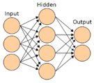
图片

一个单层前馈人工神经网络。从[math]\displaystyle{ \scriptstyle x_2 }[/math]开始的箭头为了清晰省略了。这个网络有p个输入和q个输出。在这个系统中,第q个输出的值[math]\displaystyle{ \scriptstyle {y_q} }[/math]被以[math]\displaystyle{ \scriptstyle {y_q} = K*({\sum({x_i}*{w_{iq}})}-{b_q}) }[/math]计算]]

一个两层前馈人工神经网络
一个人工神经网络

一个ANN依赖图
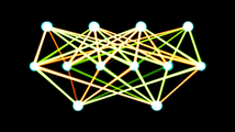
有4输入,6隐藏单元和2输出的单层前馈神经网络。给定位置状态和方向,输出转动基于控制值。
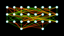
有8输入,2x8隐藏单元和2输出的两层前馈人工神经网络。给定位置状态,方向和其他环境值,输出推进基于控制值。
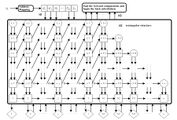
CMAC神经网络的并行流水线结构。这种学习算法可以一步收敛。


相关wiki
- 层级暂时性记忆
- 20Q
- ADALINE
- 自适应共振理论
- 人工生命
- 联合储存器
- 自编码
- BEAM机器人学
- 生物控制论
- 生物启发的计算
- 蓝脑计划
- 干涉灾难
- 小脑模型自动控制器 (CMAC)
- 认知架构
- 认知科学
- 卷积神经网络 (CNN)
- 联结主义专家系统
- 连接组
- 人工培养的神经网络
- 深度学习
- 数字形态发生
- Encog
- 模糊逻辑
- 基因表达式编程
- 遗传算法
- 遗传编程
- 数据处理的组方法
- 习惯化
- 原位自适应制表
- 机器学习概念
- 神经计算模型
- 神经进化
- 神经编码
- 神经气体
- 神经机器翻译
- 神经网络软件
- 神经科学
- Ni1000 chip
- 非线性系统识别
- 光学神经网络
- 平行-约束-满足过程
- 并行分布处理
- 径向基函数网络
- 循环神经网络
- 自组织映射
- 尖峰神经网络
- 脉动阵列
- 张量积网络
- 时延神经网络 (TDNN)
引用
- ↑ "Artificial Neural Networks as Models of Neural Information Processing, Frontiers Research Topic" (in English). Retrieved 2018-02-20.
{{cite journal}}: Cite journal requires|journal=(help) - ↑ McCulloch, Warren; Walter Pitts (1943). "A Logical Calculus of Ideas Immanent in Nervous Activity". Bulletin of Mathematical Biophysics. 5 (4): 115–133.
- ↑ Kleene, S.C. (1956). "Representation of Events in Nerve Nets and Finite Automata". Annals of Mathematics Studies (in English). Princeton University Press (34): 3–41. Retrieved 2017-06-17.
{{cite journal}}: Cite has empty unknown parameter:|dead-url=(help) - ↑ Hebb, Donald (1949). The Organization of Behavior. New York: Wiley. https://books.google.com/books?id=ddB4AgAAQBAJ.
- ↑ Farley, B.G.; W.A. Clark (1954). "Simulation of Self-Organizing Systems by Digital Computer". IRE Transactions on Information Theory. 4 (4): 76–84.
- ↑ Rochester, N.; J.H. Holland; L.H. Habit; W.L. Duda (1956). "Tests on a cell assembly theory of the action of the brain, using a large digital computer". IRE Transactions on Information Theory. 2 (3): 80–93.
- ↑ Rosenblatt, F. (1958). "The Perceptron: A Probabilistic Model For Information Storage And Organization In The Brain". Psychological Review. 65 (6): 386–408. CiteSeerX 10.1.1.588.3775.
- ↑ 8.0 8.1 Werbos, P.J. (1975). Beyond Regression: New Tools for Prediction and Analysis in the Behavioral Sciences. https://books.google.com/books?id=z81XmgEACAAJ.
- ↑ David H. Hubel and Torsten N. Wiesel (2005). Brain and visual perception: the story of a 25-year collaboration. Oxford University Press US. p. 106. https://books.google.com/books?id=8YrxWojxUA4C&pg=PA106.
- ↑ 10.0 10.1 10.2 10.3 10.4 10.5 Schmidhuber, J. (2015). "Deep Learning in Neural Networks: An Overview". Neural Networks. 61: 85–117.
- ↑ Ivakhnenko, A. G. (1973). Cybernetic Predicting Devices. CCM Information Corporation. https://books.google.com/books?id=FhwVNQAACAAJ.
- ↑ Ivakhnenko, A. G.; Grigorʹevich Lapa, Valentin (1967). Cybernetics and forecasting techniques. American Elsevier Pub. Co.. https://books.google.com/books?id=rGFgAAAAMAAJ.
- ↑ Minsky, Marvin; Papert, Seymour (1969). Perceptrons: An Introduction to Computational Geometry. MIT Press. https://books.google.com/books?id=Ow1OAQAAIAAJ.
- ↑ Rumelhart, D.E; McClelland, James (1986). Parallel Distributed Processing: Explorations in the Microstructure of Cognition. Cambridge: MIT Press. https://books.google.com/books?id=davmLgzusB8C.
- ↑ Qian, N.; Sejnowski, T.J. (1988). "Predicting the secondary structure of globular proteins using neural network models". Journal of Molecular Biology. 202: 865–884. Qian1988.
- ↑ Rost, B.; Sander, C. (1993). "Prediction of protein secondary structure at better than 70% accuracy". Journal of Molecular Biology. 232: 584–599. Rost1993.
- ↑ J. Weng, N. Ahuja and T. S. Huang, "Cresceptron: a self-organizing neural network which grows adaptively," Proc. International Joint Conference on Neural Networks, Baltimore, Maryland, vol I, pp. 576–581, June, 1992.
- ↑ 18.0 18.1 J. Weng, N. Ahuja and T. S. Huang, "Learning recognition and segmentation of 3-D objects from 2-D images," Proc. 4th International Conf. Computer Vision, Berlin, Germany, pp. 121–128, May, 1993.
- ↑ J. Weng, N. Ahuja and T. S. Huang, "Learning recognition and segmentation using the Cresceptron," International Journal of Computer Vision, vol. 25, no. 2, pp. 105–139, Nov. 1997.
- ↑ Dominik Scherer, Andreas C. Müller, and Sven Behnke: "Evaluation of Pooling Operations in Convolutional Architectures for Object Recognition," In 20th International Conference Artificial Neural Networks (ICANN), pp. 92–101, 2010.
- ↑ 21.0 21.1 S. Hochreiter., "Untersuchungen zu dynamischen neuronalen Netzen," Diploma thesis. Institut f. Informatik, Technische Univ. Munich. Advisor: J. Schmidhuber, 1991.
- ↑ Hochreiter, S.; et al. (15 January 2001). "Gradient flow in recurrent nets: the difficulty of learning long-term dependencies". A Field Guide to Dynamical Recurrent Networks. John Wiley & Sons. https://books.google.com/books?id=NWOcMVA64aAC.
- ↑ J. Schmidhuber., "Learning complex, extended sequences using the principle of history compression," Neural Computation, 4, pp. 234–242, 1992.
- ↑ Sven Behnke (2003). Hierarchical Neural Networks for Image Interpretation.. Lecture Notes in Computer Science. 2766. Springer. http://www.ais.uni-bonn.de/books/LNCS2766.pdf.
- ↑ Smolensky, P. (1986). "Information processing in dynamical systems: Foundations of harmony theory.". In D. E. Rumelhart, J. L. McClelland, & the PDP Research Group. Parallel Distributed Processing: Explorations in the Microstructure of Cognition. 1. pp. 194–281. http://portal.acm.org/citation.cfm?id=104290.
- ↑ 26.0 26.1 26.2 Hinton, G. E.; Osindero, S.; Teh, Y. (2006). "A fast learning algorithm for deep belief nets" (PDF). Neural Computation. 18 (7): 1527–1554.
{{cite journal}}: External link in|journal= - ↑ Hinton, G. (2009). "Deep belief networks". Scholarpedia. 4 (5): 5947.
- ↑ Ng, Andrew; Dean, Jeff (2012). "Building High-level Features Using Large Scale Unsupervised Learning".
{{cite journal}}: Cite journal requires|journal=(help); Unknown parameter|class=ignored (help) - ↑ Yang, J. J.; Pickett, M. D.; Li, X. M.; Ohlberg, D. A. A.; Stewart, D. R.; Williams, R. S. (2008). "Memristive switching mechanism for metal/oxide/metal nanodevices". Nat. Nanotechnol. 3 (7): 429–433.
- ↑ Strukov, D. B.; Snider, G. S.; Stewart, D. R.; Williams, R. S. (2008). "The missing memristor found". Nature. 453 (7191): 80–83.
- ↑ Cireşan, Dan Claudiu; Meier, Ueli; Gambardella, Luca Maria; Schmidhuber, Jürgen (2010-09-21). "Deep, Big, Simple Neural Nets for Handwritten Digit Recognition". Neural Computation. 22 (12): 3207–3220.
- ↑ 2012 Kurzweil AI Interview with Jürgen Schmidhuber on the eight competitions won by his Deep Learning team 2009–2012
- ↑ "How bio-inspired deep learning keeps winning competitions, KurzweilAI". www.kurzweilai.net (in English). Retrieved 2017-06-16.
{{cite journal}}: Cite has empty unknown parameter:|dead-url=(help) - ↑ Graves, Alex; and Schmidhuber, Jürgen; Offline Handwriting Recognition with Multidimensional Recurrent Neural Networks, in Bengio, Yoshua; Schuurmans, Dale; Lafferty, John; Williams, Chris K. I.; and Culotta, Aron (eds.), Advances in Neural Information Processing Systems 22 (NIPS'22), 7–10 December 2009, Vancouver, BC, Neural Information Processing Systems (NIPS) Foundation, 2009, pp. 545–552.
- ↑ 35.0 35.1 Graves, A.; Liwicki, M.; Fernandez, S.; Bertolami, R.; Bunke, H.; Schmidhuber, J. (2009). "A Novel Connectionist System for Improved Unconstrained Handwriting Recognition" (PDF). IEEE Transactions on Pattern Analysis and Machine Intelligence. 31 (5): 855–868.
- ↑ 36.0 36.1 36.2 Graves, Alex; Schmidhuber, Jürgen (2009). Bengio, Yoshua; Schuurmans, Dale; Lafferty, John; Williams, Chris editor-K. I.; Culotta, Aron (eds.). "Offline Handwriting Recognition with Multidimensional Recurrent Neural Networks". Neural Information Processing Systems (NIPS) Foundation: 545–552.
{{cite journal}}:|editor-first4=has generic name (help) - ↑ Graves, A.; Liwicki, M.; Fernández, S.; Bertolami, R.; Bunke, H.; Schmidhuber, J. (May 2009). "A Novel Connectionist System for Unconstrained Handwriting Recognition". IEEE Transactions on Pattern Analysis and Machine Intelligence. 31 (5): 855–868.
- ↑ 38.0 38.1 Cireşan, Dan; Meier, Ueli; Masci, Jonathan; Schmidhuber, Jürgen (August 2012). "Multi-column deep neural network for traffic sign classification". Neural Networks. Selected Papers from IJCNN 2011. 32: 333–338.
- ↑ 39.0 39.1 Ciresan, Dan; Giusti, Alessandro; Gambardella, Luca M.; Schmidhuber, Juergen (2012). Pereira, F.. ed. Advances in Neural Information Processing Systems 25. Curran Associates, Inc.. pp. 2843–2851. http://papers.nips.cc/paper/4741-deep-neural-networks-segment-neuronal-membranes-in-electron-microscopy-images.pdf.
- ↑ 40.0 40.1 Ciresan, Dan; Meier, U.; Schmidhuber, J. (June 2012). "Multi-column deep neural networks for image classification". 2012 IEEE Conference on Computer Vision and Pattern Recognition: 3642–3649.
- ↑ 41.0 41.1 Ciresan, D. C.; Meier, U.; Masci, J.; Gambardella, L. M.; Schmidhuber, J. (2011). "Flexible, High Performance Convolutional Neural Networks for Image Classification" (PDF). International Joint Conference on Artificial Intelligence.
- ↑ Krizhevsky, Alex; Sutskever, Ilya; Hinton, Geoffry (2012). "ImageNet Classification with Deep Convolutional Neural Networks" (PDF). NIPS 2012: Neural Information Processing Systems, Lake Tahoe, Nevada.
- ↑ Fukushima, K. (1980). "Neocognitron: A self-organizing neural network model for a mechanism of pattern recognition unaffected by shift in position". Biological Cybernetics. 36 (4): 93–202.
- ↑ Riesenhuber, M; Poggio, T (1999). "Hierarchical models of object recognition in cortex". Nature Neuroscience. 2 (11): 1019–1025.
- ↑ Hinton, Geoffrey (2009-05-31). "Deep belief networks". Scholarpedia (in English). 4 (5): 5947.
- ↑ Markoff, John (November 23, 2012). "Scientists See Promise in Deep-Learning Programs". New York Times.
- ↑ Martines, H.; Bengio, Y.; Yannakakis, G. N. (2013). "Learning Deep Physiological Models of Affect". IEEE Computational Intelligence. 8 (2): 20–33.
- ↑ J. Weng, "Why Have We Passed 'Neural Networks Do not Abstract Well'?," Natural Intelligence: the INNS Magazine, vol. 1, no.1, pp. 13–22, 2011.
- ↑ Z. Ji, J. Weng, and D. Prokhorov, "Where-What Network 1: Where and What Assist Each Other Through Top-down Connections," Proc. 7th International Conference on Development and Learning (ICDL'08), Monterey, CA, Aug. 9–12, pp. 1–6, 2008.
- ↑ X. Wu, G. Guo, and J. Weng, "Skull-closed Autonomous Development: WWN-7 Dealing with Scales," Proc. International Conference on Brain-Mind, July 27–28, East Lansing, Michigan, pp. 1–9, 2013.
- ↑ 51.0 51.1 51.2 51.3 51.4 Zell, Andreas (1994). "chapter 5.2" (in German). Simulation Neuronaler Netze (1st ed.). Addison-Wesley.
- ↑ Abbod, Maysam F (2007). "Application of Artificial Intelligence to the Management of Urological Cancer". The Journal of Urology. 178 (4): 1150–1156.
- ↑ DAWSON, CHRISTIAN W (1998). "An artificial neural network approach to rainfall-runoff modelling". Hydrological Sciences Journal. 43 (1): 47–66.
- ↑ "The Machine Learning Dictionary".
{{cite journal}}: Cite journal requires|journal=(help) - ↑ 55.0 55.1 55.2 55.3 Schmidhuber, Jürgen (2015). "Deep Learning". Scholarpedia. 10 (11): 32832.
- ↑ Dreyfus, Stuart E. (1990-09-01). "Artificial neural networks, back propagation, and the Kelley-Bryson gradient procedure". Journal of Guidance, Control, and Dynamics. 13 (5): 926–928.
- ↑ Eiji Mizutani, Stuart Dreyfus, Kenichi Nishio (2000). On derivation of MLP backpropagation from the Kelley-Bryson optimal-control gradient formula and its application. Proceedings of the IEEE International Joint Conference on Neural Networks (IJCNN 2000), Como Italy, July 2000. Online
- ↑ Kelley, Henry J. (1960). "Gradient theory of optimal flight paths". Ars Journal. 30 (10): 947–954.
- ↑ Arthur E. Bryson (1961, April). A gradient method for optimizing multi-stage allocation processes. In Proceedings of the Harvard Univ. Symposium on digital computers and their applications.
- ↑ Dreyfus, Stuart (1962). "The numerical solution of variational problems". Journal of Mathematical Analysis and Applications. 5 (1): 30–45.
- ↑ Russell, Stuart J.; Norvig, Peter (2010). Artificial Intelligence A Modern Approach. Prentice Hall. p. 578. https://books.google.com/books?id=8jZBksh-bUMC&pg=PA578. "The most popular method for learning in multilayer networks is called Back-propagation."
- ↑ Bryson, Arthur Earl (1969). Applied Optimal Control: Optimization, Estimation and Control. Blaisdell Publishing Company or Xerox College Publishing. p. 481. https://books.google.com/books?id=1bChDAEACAAJ&pg=PA481.
- ↑ Seppo Linnainmaa (1970). The representation of the cumulative rounding error of an algorithm as a Taylor expansion of the local rounding errors. Master's Thesis (in Finnish), Univ. Helsinki, 6–7.
- ↑ Linnainmaa, Seppo (1976). "Taylor expansion of the accumulated rounding error". BIT Numerical Mathematics. 16 (2): 146–160.
- ↑ Griewank, Andreas (2012). "Who Invented the Reverse Mode of Differentiation?" (PDF). Documenta Matematica, Extra Volume ISMP: 389–400.
- ↑ Griewank, Andreas; Walther, Andrea (2008). Evaluating Derivatives: Principles and Techniques of Algorithmic Differentiation, Second Edition. SIAM. https://books.google.com/books?id=xoiiLaRxcbEC.
- ↑ Dreyfus, Stuart (1973). "The computational solution of optimal control problems with time lag". IEEE Transactions on Automatic Control. 18 (4): 383–385.
- ↑ https://en.wikipedia.org/wiki/Paul_Werbos (1974). Beyond regression: New tools for prediction and analysis in the behavioral sciences. PhD thesis, Harvard University.
- ↑ Werbos, Paul (1982). "Applications of advances in nonlinear sensitivity analysis". System modeling and optimization. Springer. pp. 762–770. http://werbos.com/Neural/SensitivityIFIPSeptember1981.pdf.
- ↑ Rumelhart, David E.; Hinton, Geoffrey E.; Williams, Ronald J. (1986). "Learning representations by back-propagating errors". Nature. 323 (6088): 533–536.
- ↑ Eric A. Wan (1993). "Time series prediction by using a connectionist network with internal delay lines." In Proceedings of the Santa Fe Institute Studies in the Sciences of Complexity, 15: p. 195. Addison-Wesley Publishing Co.
- ↑ Hinton, G.; Deng, L.; Yu, D.; Dahl, G. E.; Mohamed, A. r; Jaitly, N.; Senior, A.; Vanhoucke, V.; Nguyen, P. (November 2012). "Deep Neural Networks for Acoustic Modeling in Speech Recognition: The Shared Views of Four Research Groups". IEEE Signal Processing Magazine. 29 (6): 82–97.
- ↑ Huang, Guang-Bin; Zhu, Qin-Yu; Siew, Chee-Kheong (2006). "Extreme learning machine: theory and applications". Neurocomputing. 70 (1): 489–501.
- ↑ Ollivier, Yann; Charpiat, Guillaume (2015). "Training recurrent networks without backtracking".
{{cite journal}}: Cite journal requires|journal=(help) - ↑ ESANN. 2009
- ↑ Hinton, G. E. (2010). "A Practical Guide to Training Restricted Boltzmann Machines". Tech. Rep. UTML TR 2010-003,.
{{cite journal}}: CS1 maint: extra punctuation (link) - ↑ Widrow, Bernard; et al. (2013). "The no-prop algorithm: A new learning algorithm for multilayer neural networks". Neural Networks. 37: 182–188.
- ↑ Ojha, Varun Kumar; Abraham, Ajith; Snášel, Václav (2017-04-01). "Metaheuristic design of feedforward neural networks: A review of two decades of research". Engineering Applications of Artificial Intelligence. 60: 97–116.
- ↑ Dominic, S.; Das, R.; Whitley, D.; Anderson, C. (July 1991). "Genetic reinforcement learning for neural networks". IJCNN-91-Seattle International Joint Conference on Neural Networks. Seattle, Washington, USA: IEEE.
- ↑ Hoskins, J.C.; Himmelblau, D.M. (1992). "Process control via artificial neural networks and reinforcement learning". Computers & Chemical Engineering. 16 (4): 241–251.
- ↑ Bertsekas, D.P.; Tsitsiklis, J.N. (1996). Neuro-dynamic programming. Athena Scientific. p. 512. https://papers.nips.cc/paper/4741-deep-neural-networks-segment-neuronal-membranes-in-electron-microscopy-images.
- ↑ Secomandi, Nicola (2000). "Comparing neuro-dynamic programming algorithms for the vehicle routing problem with stochastic demands". Computers & Operations Research. 27 (11–12): 1201–1225.
- ↑ de Rigo, D.; Rizzoli, A. E.; Soncini-Sessa, R.; Weber, E.; Zenesi, P. (2001). "Neuro-dynamic programming for the efficient management of reservoir networks" (PDF). MODSIM 2001, International Congress on Modelling and Simulation. Canberra, Australia: Modelling and Simulation Society of Australia and New Zealand. Retrieved 29 July 2012.
- ↑ Damas, M.; Salmeron, M.; Diaz, A.; Ortega, J.; Prieto, A.; Olivares, G. (2000). "Genetic algorithms and neuro-dynamic programming: application to water supply networks". 2000 Congress on Evolutionary Computation. La Jolla, California, USA: IEEE.
- ↑ Deng, Geng; Ferris, M.C. (2008). "Neuro-dynamic programming for fractionated radiotherapy planning". Springer Optimization and Its Applications. Springer Optimization and Its Applications. 12: 47–70. CiteSeerX 10.1.1.137.8288.
- ↑ M. Forouzanfar; H. R. Dajani; V. Z. Groza; M. Bolic; S. Rajan (July 2010). "Comparison of Feed-Forward Neural Network Training Algorithms for Oscillometric Blood Pressure Estimation" (PDF). 4th Int. Workshop Soft Computing Applications. Arad, Romania: IEEE.
{{cite journal}}: Unknown parameter|last-author-amp=ignored (help) - ↑ de Rigo, D.; Castelletti, A.; Rizzoli, A. E.; Soncini-Sessa, R.; Weber, E. (January 2005). Pavel Zítek (ed.). "A selective improvement technique for fastening Neuro-Dynamic Programming in Water Resources Network Management". 16th IFAC World Congress. Prague, Czech Republic: IFAC. 16. Retrieved 30 December 2011.
- ↑ Ferreira, C. (2006). "Designing Neural Networks Using Gene Expression Programming" (PDF). In A. Abraham, B. de Baets, M. Köppen, and B. Nickolay, eds., Applied Soft Computing Technologies: The Challenge of Complexity, pages 517–536, Springer-Verlag.
{{cite journal}}: Cite journal requires|journal=(help) - ↑ Da, Y.; Xiurun, G. (July 2005). T. Villmann (ed.). "An improved PSO-based ANN with simulated annealing technique". New Aspects in Neurocomputing: 11th European Symposium on Artificial Neural Networks. Elsevier.
- ↑ Wu, J.; Chen, E. (May 2009). "A Novel Nonparametric Regression Ensemble for Rainfall Forecasting Using Particle Swarm Optimization Technique Coupled with Artificial Neural Network". 6th International Symposium on Neural Networks, ISNN 2009. Springer.
{{cite journal}}: Unknown parameter|editors=ignored (help) - ↑ 91.0 91.1 91.2 Ting Qin, et al. "A learning algorithm of CMAC based on RLS." Neural Processing Letters 19.1 (2004): 49–61.
- ↑ Ting Qin, et al. "Continuous CMAC-QRLS and its systolic array." Neural Processing Letters 22.1 (2005): 1–16.
- ↑ Ivakhnenko, Alexey Grigorevich (1968). "The group method of data handling – a rival of the method of stochastic approximation". Soviet Automatic Control. 13 (3): 43–55.
- ↑ Ivakhnenko, Alexey (1971). "Polynomial theory of complex systems". IEEE Transactions on Systems, Man and Cybernetics (4) (4): 364–378.
- ↑ Kondo, T.; Ueno, J. (2008). "Multi-layered GMDH-type neural network self-selecting optimum neural network architecture and its application to 3-dimensional medical image recognition of blood vessels". International Journal of Innovative Computing, Information and Control. 4 (1): 175–187.
- ↑ Fukushima, K. (1980). "Neocognitron: A self-organizing neural network model for a mechanism of pattern recognition unaffected by shift in position". Biol. Cybern. 36 (4): 193–202.
- ↑ LeCun et al., "Backpropagation Applied to Handwritten Zip Code Recognition," Neural Computation, 1, pp. 541–551, 1989.
- ↑ Yann LeCun (2016). Slides on Deep Learning Online
- ↑ "Unsupervised Feature Learning and Deep Learning Tutorial".
{{cite journal}}: Cite journal requires|journal=(help) - ↑ Szegedy, Christian; Liu, Wei; Jia, Yangqing; Sermanet, Pierre; Reed, Scott; Anguelov, Dragomir; Erhan, Dumitru; Vanhoucke, Vincent; Rabinovich, Andrew (2014). "Going Deeper with Convolutions". Computing Research Repository: 1.
- ↑ Ran, Lingyan; Zhang, Yanning; Zhang, Qilin; Yang, Tao (2017-06-12). "Convolutional Neural Network-Based Robot Navigation Using Uncalibrated Spherical Images" (PDF). Sensors. MDPI AG. 17 (6): 1341.
- ↑ Hochreiter, Sepp; Schmidhuber, Jürgen (1997-11-01). "Long Short-Term Memory". Neural Computation. 9 (8): 1735–1780.
- ↑ "Learning Precise Timing with LSTM Recurrent Networks (PDF Download Available)". ResearchGate (in English): 115–143. Retrieved 2017-06-13.
- ↑ Bayer, Justin; Wierstra, Daan; Togelius, Julian; Schmidhuber, Jürgen (2009-09-14). "Evolving Memory Cell Structures for Sequence Learning". Artificial Neural Networks – ICANN 2009. Lecture Notes in Computer Science (in English). Springer, Berlin, Heidelberg. 5769: 755–764.
- ↑ Fernández, Santiago; Graves, Alex; Schmidhuber, Jürgen (2007). "Sequence labelling in structured domains with hierarchical recurrent neural networks". In Proc. 20th Int. Joint Conf. on Artificial In℡ligence, Ijcai 2007: 774–779.
- ↑ Graves, Alex; Fernández, Santiago; Gomez, Faustino (2006). "Connectionist temporal classification: Labelling unsegmented sequence data with recurrent neural networks". In Proceedings of the International Conference on Machine Learning, ICML 2006: 369–376.
- ↑ Graves, Alex; Eck, Douglas; Beringer, Nicole; Schmidhuber, Jürgen (2003). "Biologically Plausible Speech Recognition with LSTM Neural Nets" (PDF). 1st Intl. Workshop on Biologically Inspired Approaches to Advanced Information Technology, Bio-ADIT 2004, Lausanne, Switzerland: 175–184.
{{cite journal}}: Cite has empty unknown parameter:|dead-url=(help) - ↑ Fernández, Santiago; Graves, Alex; Schmidhuber, Jürgen (2007). "An Application of Recurrent Neural Networks to Discriminative Keyword Spotting". Proceedings of the 17th International Conference on Artificial Neural Networks. ICANN'07. Berlin, Heidelberg: Springer-Verlag: 220–229.
- ↑ Hannun, Awni; Case, Carl; Casper, Jared; Catanzaro, Bryan; Diamos, Greg; Elsen, Erich; Prenger, Ryan; Satheesh, Sanjeev; Sengupta, Shubho (2014-12-17). "Deep Speech: Scaling up end-to-end speech recognition".
{{cite journal}}: Cite journal requires|journal=(help) - ↑ Sak, Hasim; Senior, Andrew; Beaufays, Francoise (2014). "Long Short-Term Memory recurrent neural network architectures for large scale acoustic modeling" (PDF).
{{cite journal}}: Cite journal requires|journal=(help); Cite has empty unknown parameter:|dead-url=(help) - ↑ Li, Xiangang; Wu, Xihong (2014-10-15). "Constructing Long Short-Term Memory based Deep Recurrent Neural Networks for Large Vocabulary Speech Recognition".
{{cite journal}}: Cite journal requires|journal=(help) - ↑ Fan, Y.; Qian, Y.; Xie, F.; Soong, F. K. (2014). "TTS synthesis with bidirectional LSTM based Recurrent Neural Networks". ResearchGate (in English). Retrieved 2017-06-13.
{{cite journal}}: Cite has empty unknown parameter:|dead-url=(help) - ↑ Zen, Heiga; Sak, Hasim (2015). "Unidirectional Long Short-Term Memory Recurrent Neural Network with Recurrent Output Layer for Low-Latency Speech Synthesis" (PDF). Google.com. ICASSP: 4470–4474.
{{cite journal}}: Cite has empty unknown parameter:|dead-url=(help) - ↑ Fan, Bo; Wang, Lijuan; Soong, Frank K.; Xie, Lei (2015). "Photo-Real Talking Head with Deep Bidirectional LSTM" (PDF). Proceedings of ICASSP.
- ↑ Sak, Haşim; Senior, Andrew; Rao, Kanishka; Beaufays, Françoise; Schalkwyk, Johan (September 2015). "Google voice search: faster and more accurate".
{{cite journal}}: Cite journal requires|journal=(help); Cite has empty unknown parameter:|dead-url=(help) - ↑ Gers, Felix A.; Schmidhuber, Jürgen (2001). "LSTM Recurrent Networks Learn Simple Context Free and Context Sensitive Languages". IEEE Transactions on Neural Networks. 12 (6): 1333–1340.
- ↑ Huang, Jie; Zhou, Wengang; Zhang, Qilin; Li, Houqiang; Li, Weiping (2018-01-30). "Video-based Sign Language Recognition without Temporal Segmentation" (PDF).
{{cite journal}}: Cite journal requires|journal=(help) - ↑ Sutskever, L.; Vinyals, O.; Le, Q. (2014). "Sequence to Sequence Learning with Neural Networks". NIPS'14 Proceedings of the 27th International Conference on Neural Information Processing Systems. 2: 3104–3112.
- ↑ Jozefowicz, Rafal; Vinyals, Oriol; Schuster, Mike; Shazeer, Noam; Wu, Yonghui (2016-02-07). "Exploring the Limits of Language Modeling".
{{cite journal}}: Cite journal requires|journal=(help) - ↑ Gillick, Dan; Brunk, Cliff; Vinyals, Oriol; Subramanya, Amarnag (2015-11-30). "Multilingual Language Processing From Bytes".
{{cite journal}}: Cite journal requires|journal=(help) - ↑ Vinyals, Oriol; Toshev, Alexander; Bengio, Samy; Erhan, Dumitru (2014-11-17). "Show and Tell: A Neural Image Caption Generator".
{{cite journal}}: Cite journal requires|journal=(help) - ↑ Gallicchio, Claudio; Micheli, Alessio; Pedrelli, Luca (2017). "Deep reservoir computing: A critical experimental analysis". Neurocomputing. 268: 87.
- ↑ Gallicchio, Claudio; Micheli, Alessio (2017). "Echo State Property of Deep Reservoir Computing Networks". Cognitive Computation (in English). 9 (3): 337–350.
- ↑ Hinton, G.E. (2009). "Deep belief networks". Scholarpedia. 4 (5): 5947.
- ↑ Larochelle, Hugo; Erhan, Dumitru; Courville, Aaron; Bergstra, James; Bengio, Yoshua (2007). "An Empirical Evaluation of Deep Architectures on Problems with Many Factors of Variation". Proceedings of the 24th International Conference on Machine Learning. ICML '07. New York, NY, USA: ACM: 473–480.
- ↑ 126.0 126.1 Graupe, Daniel (2013). Principles of Artificial Neural Networks. World Scientific. pp. 1–. https://books.google.com/books?id=W6W6CgAAQBAJ&pg=PP1.
- ↑ Graupe, Daniel (2016). "Large memory storage and retrieval(LAMSTAR) network".
{{cite journal}}: Cite journal requires|journal=(help) - ↑ D. Graupe, "Principles of Artificial Neural Networks.3rd Edition", World Scientific Publishers, 2013, pp. 203–274.
- ↑ Nigam, Vivek Prakash; Graupe, Daniel (2004-01-01). "A neural-network-based detection of epilepsy". Neurological Research. 26 (1): 55–60.
- ↑ 130.0 130.1 Waxman, Jonathan A.; Graupe, Daniel; Carley, David W. (2010-04-01). "Automated Prediction of Apnea and Hypopnea, Using a LAMSTAR Artificial Neural Network". American Journal of Respiratory and Critical Care Medicine. 181 (7): 727–733.
- ↑ 131.0 131.1 Graupe, D.; Graupe, M. H.; Zhong, Y.; Jackson, R. K. (2008). "Blind adaptive filtering for non-invasive extraction of the fetal electrocardiogram and its non-stationarities". Proc. Inst. Mech. Eng. H. 222 (8): 1221–1234.
- ↑ Graupe 2013" "pp=240–253"
- ↑ 133.0 133.1 Graupe, D.; Abon, J. (2002). "A Neural Network for Blind Adaptive Filtering of Unknown Noise from Speech". Intelligent Engineering Systems Through Artificial Neural Networks (in English). Technische Informationsbibliothek (TIB). 12: 683–688. Retrieved 2017-06-14.
- ↑ D. Graupe, "Principles of Artificial Neural Networks.3rd Edition", World Scientific Publishers", 2013, pp. 253–274.
- ↑ Girado, J. I.; Sandin, D. J.; DeFanti, T. A. (2003). "Real-time camera-based face detection using a modified LAMSTAR neural network system". Proc. SPIE 5015, Applications of Artificial Neural Networks in Image Processing VIII. Applications of Artificial Neural Networks in Image Processing VIII. 5015: 36.
- ↑ Venkatachalam, V; Selvan, S. (2007). "Intrusion Detection using an Improved Competitive Learning Lamstar Network". International Journal of Computer Science and Network Security. 7 (2): 255–263.
- ↑ Graupe, D.; Smollack, M. (2007). "Control of unstable nonlinear and nonstationary systems using LAMSTAR neural networks". ResearchGate (in English). Proceedings of 10th IASTED on Intelligent Control, Sect.592,: 141–144. Retrieved 2017-06-14.
{{cite journal}}: Cite has empty unknown parameter:|dead-url=(help)CS1 maint: extra punctuation (link) - ↑ Graupe, Daniel (7 July 2016). Deep Learning Neural Networks: Design and Case Studies. World Scientific Publishing Co Inc. pp. 57–110. https://books.google.com/books?id=e5hIDQAAQBAJ&pg=PA57.
- ↑ Graupe, D.; Kordylewski, H. (August 1996). "Network based on SOM (Self-Organizing-Map) modules combined with statistical decision tools". Proceedings of the 39th Midwest Symposium on Circuits and Systems. 1: 471–474 vol.1.
- ↑ Graupe, D.; Kordylewski, H. (1998-03-01). "A Large Memory Storage and Retrieval Neural Network for Adaptive Retrieval and Diagnosis". International Journal of Software Engineering and Knowledge Engineering. 08 (1): 115–138.
- ↑ Kordylewski, H.; Graupe, D; Liu, K. (2001). "A novel large-memory neural network as an aid in medical diagnosis applications". IEEE Transactions on Information Technology in Biomedicine. 5 (3): 202–209.
- ↑ Schneider, N.C.; Graupe (2008). "A modified LAMSTAR neural network and its applications". International journal of neural systems. 18 (4): 331–337.
- ↑ "Graupe 2013" "p=217"
- ↑ 144.0 144.1 144.2 144.3 Vincent, Pascal; Larochelle, Hugo; Lajoie, Isabelle; Bengio, Yoshua; Manzagol, Pierre-Antoine (2010). "Stacked Denoising Autoencoders: Learning Useful Representations in a Deep Network with a Local Denoising Criterion". The Journal of Machine Learning Research. 11: 3371–3408.
- ↑ Ballard, Dana H. (1987). "Modular learning in neural networks" (PDF). Proceedings of AAAI: 279–284.
{{cite journal}}: Cite has empty unknown parameter:|dead-url=(help) - ↑ 146.0 146.1 146.2 Deng, Li; Yu, Dong; Platt, John (2012). "Scalable stacking and learning for building deep architectures" (PDF). 2012 IEEE International Conference on Acoustics, Speech and Signal Processing (ICASSP): 2133–2136.
- ↑ 147.0 147.1 Deng, Li; Yu, Dong (2011). "Deep Convex Net: A Scalable Architecture for Speech Pattern Classification" (PDF). Proceedings of the Interspeech: 2285–2288.
- ↑ David, Wolpert (1992). "Stacked generalization". Neural Networks. 5 (2): 241–259.
- ↑ Bengio, Y. (2009-11-15). "Learning Deep Architectures for AI". Foundations and Trends® in Machine Learning (in English). 2 (1): 1–127.
- ↑ Hutchinson, Brian; Deng, Li; Yu, Dong (2012). "Tensor deep stacking networks". IEEE Transactions on Pattern Analysis and Machine Intelligence. 1–15 (8): 1944–1957.
- ↑ Hinton, Geoffrey; Salakhutdinov, Ruslan (2006). "Reducing the Dimensionality of Data with Neural Networks". Science. 313 (5786): 504–507.
- ↑ Dahl, G.; Yu, D.; Deng, L.; Acero, A. (2012). "Context-Dependent Pre-Trained Deep Neural Networks for Large-Vocabulary Speech Recognition". IEEE Transactions on Audio, Speech, and Language Processing. 20 (1): 30–42.
- ↑ Mohamed, Abdel-rahman; Dahl, George; Hinton, Geoffrey (2012). "Acoustic Modeling Using Deep Belief Networks". IEEE Transactions on Audio, Speech, and Language Processing. 20 (1): 14–22.
- ↑ Courville, Aaron; Bergstra, James; Bengio, Yoshua (2011). "A Spike and Slab Restricted Boltzmann Machine" (PDF). JMLR: Workshop and Conference Proceeding. 15: 233–241.
- ↑ 155.0 155.1 Courville, Aaron; Bergstra, James; Bengio, Yoshua (2011). "Unsupervised Models of Images by Spike-and-Slab RBMs" (PDF). Proceedings of the 28th International Conference on Machine Learning. 10: 1–8.
- ↑ Mitchell, T; Beauchamp, J (1988). "Bayesian Variable Selection in Linear Regression". Journal of the American Statistical Association. 83 (404): 1023–1032.
- ↑ Hinton, Geoffrey; Salakhutdinov, Ruslan (2009). "Efficient Learning of Deep Boltzmann Machines" (PDF). 3: 448–455.
{{cite journal}}: Cite journal requires|journal=(help) - ↑ Larochelle, Hugo; Bengio, Yoshua; Louradour, Jerdme; Lamblin, Pascal (2009). "Exploring Strategies for Training Deep Neural Networks". The Journal of Machine Learning Research. 10: 1–40.
- ↑ Coates, Adam; Carpenter, Blake (2011). "Text Detection and Character Recognition in Scene Images with Unsupervised Feature Learning" (PDF): 440–445.
{{cite journal}}: Cite journal requires|journal=(help) - ↑ Lee, Honglak; Grosse, Roger (2009). "Convolutional deep belief networks for scalable unsupervised learning of hierarchical representations". Proceedings of the 26th Annual International Conference on Machine Learning: 1–8.
- ↑ Lin, Yuanqing; Zhang, Tong (2010). "Deep Coding Network" (PDF). Advances in Neural . . .: 1–9.
- ↑ Ranzato, Marc Aurelio; Boureau, Y-Lan (2007). "Sparse Feature Learning for Deep Belief Networks" (PDF). Advances in Neural Information Processing Systems. 23: 1–8.
- ↑ Socher, Richard; Lin, Clif (2011). "Parsing Natural Scenes and Natural Language with Recursive Neural Networks" (PDF). Proceedings of the 26th International Conference on Machine Learning.
- ↑ Taylor, Graham; Hinton, Geoffrey (2006). "Modeling Human Motion Using Binary Latent Variables" (PDF). Advances in Neural Information Processing Systems.
- ↑ Vincent, Pascal; Larochelle, Hugo (2008). "Extracting and composing robust features with denoising autoencoders". Proceedings of the 25th international conference on Machine learning – ICML '08: 1096–1103.
- ↑ Kemp, Charles; Perfors, Amy; Tenenbaum, Joshua (2007). "Learning overhypotheses with hierarchical Bayesian models". Developmental Science. 10 (3): 307–21.
- ↑ Xu, Fei; Tenenbaum, Joshua (2007). "Word learning as Bayesian inference". Psychol. Rev. 114 (2): 245–72.
- ↑ Chen, Bo; Polatkan, Gungor (2011). "The Hierarchical Beta Process for Convolutional Factor Analysis and Deep Learning" (PDF). Machine Learning . . .
- ↑ Fei-Fei, Li; Fergus, Rob (2006). "One-shot learning of object categories". IEEE Transactions on Pattern Analysis and Machine Intelligence. 28 (4): 594–611.
- ↑ Rodriguez, Abel; Dunson, David (2008). "The Nested Dirichlet Process". Journal of the American Statistical Association. 103 (483): 1131–1154.
- ↑ Ruslan, Salakhutdinov; Joshua, Tenenbaum (2012). "Learning with Hierarchical-Deep Models". IEEE Transactions on Pattern Analysis and Machine Intelligence. 35 (8): 1958–71.
- ↑ 172.0 172.1 Chalasani, Rakesh; Principe, Jose (2013). "Deep Predictive Coding Networks".
{{cite journal}}: Cite journal requires|journal=(help) - ↑ Hinton, Geoffrey E. (1984). "Distributed representations".
{{cite journal}}: Cite journal requires|journal=(help); Cite has empty unknown parameter:|dead-url=(help) - ↑ S. Das, C.L. Giles, G.Z. Sun, "Learning Context Free Grammars: Limitations of a Recurrent Neural Network with an External Stack Memory," Proc. 14th Annual Conf. of the Cog. Sci. Soc., p. 79, 1992.
- ↑ Mozer, M. C.; Das, S. (1993). "A connectionist symbol manipulator that discovers the structure of context-free languages". NIPS 5: 863–870.
{{cite journal}}: Cite journal requires|journal=(help); Cite has empty unknown parameter:|dead-url=(help) - ↑ Schmidhuber, J. (1992). "Learning to control fast-weight memories: An alternative to recurrent nets". Neural Computation. 4 (1): 131–139.
- ↑ Gers, F.; Schraudolph, N.; Schmidhuber, J. (2002). "Learning precise timing with LSTM recurrent networks" (PDF). JMLR. 3: 115–143.
- ↑ Jürgen Schmidhuber (1993). "An introspective network that can learn to run its own weight change algorithm". In Proc. of the Intl. Conf. on Artificial Neural Networks, Brighton. IEE: 191–195.
{{cite journal}}: External link in|author= - ↑ Hochreiter, Sepp; Younger, A. Steven; Conwell, Peter R. (2001). "Learning to Learn Using Gradient Descent". ICANN. 2130: 87–94.
- ↑ Grefenstette, Edward, et al. "Learning to Transduce with Unbounded Memory."(2015).
- ↑ Graves, Alex, Greg Wayne, and Ivo Danihelka. "Neural Turing Machines." (2014).
- ↑ Burgess, Matt. "DeepMind's AI learned to ride the London Underground using human-like reason and memory". WIRED UK (in British English). Retrieved 2016-10-19.
- ↑ "DeepMind AI 'Learns' to Navigate London Tube". PCMAG. Retrieved 2016-10-19.
- ↑ Mannes, John. "DeepMind's differentiable neural computer helps you navigate the subway with its memory". TechCrunch. Retrieved 2016-10-19.
- ↑ Graves, Alex; Wayne, Greg; Reynolds, Malcolm; Harley, Tim; Danihelka, Ivo; Grabska-Barwińska, Agnieszka; Colmenarejo, Sergio Gómez; Grefenstette, Edward; Ramalho, Tiago (2016-10-12). "Hybrid computing using a neural network with dynamic external memory". Nature (in English). 538 (7626): 471–476.
- ↑ "Differentiable neural computers, DeepMind". DeepMind. Retrieved 2016-10-19.
- ↑ Atkeson, Christopher G.; Schaal, Stefan (1995). "Memory-based neural networks for robot learning". Neurocomputing. 9 (3): 243–269.
- ↑ Salakhutdinov, Ruslan, and Geoffrey Hinton. "Semantic hashing." International Journal of Approximate Reasoning 50.7 (2009): 969–978.
- ↑ Le, Quoc V.; Mikolov, Tomas (2014). "Distributed representations of sentences and documents".
{{cite journal}}: Cite journal requires|journal=(help) - ↑ Weston, Jason, Sumit Chopra, and Antoine Bordes. "Memory networks." (2014).
- ↑ Sukhbaatar, Sainbayar, et al. "End-To-End Memory Networks."(2015).
- ↑ Bordes, Antoine, et al. "Large-scale Simple Question Answering with Memory Networks." (2015).
- ↑ "AI device identifies objects at the speed of light: The 3D-printed artificial neural network can be used in medicine, robotics and security". ScienceDaily (in English). Retrieved 2018-08-08.
- ↑ Vinyals, Oriol, Meire Fortunato, and Navdeep Jaitly. "Pointer networks."(2015).
- ↑ Kurach, Karol, Andrychowicz, Marcin and Sutskever, Ilya."Neural Random-Access Machines."(2015).
- ↑ Kalchbrenner, N.; Blunsom, P. (2013). "Recurrent continuous translation models". EMNLP'2013.
{{cite journal}}: Cite journal requires|journal=(help); Cite has empty unknown parameter:|dead-url=(help) - ↑ Sutskever, I.; Vinyals, O.; Le, Q. V. (2014). "Sequence to sequence learning with neural networks" (PDF). NIPS'2014.
{{cite journal}}: Cite journal requires|journal=(help); Cite has empty unknown parameter:|dead-url=(help) - ↑ Cho, K.; van Merrienboer, B.; Gulcehre, C.; Bougares, F.; Schwenk, H.; Bengio, Y. (October 2014). "Learning phrase representations using RNN encoder-decoder for statistical machine translation". Proceedings of the Empiricial Methods in Natural Language Processing. 1406: arXiv:1406.1078.
- ↑ Cho, Kyunghyun, Aaron Courville, and Yoshua Bengio."Describing Multimedia Content using Attention-based Encoder–Decoder Networks." (2015).
- ↑ Scholkopf, B; Smola, Alexander (1998). "Nonlinear component analysis as a kernel eigenvalue problem". Neural computation. (44) (5): 1299–1319. CiteSeerX 10.1.1.53.8911.
- ↑ Cho, Youngmin (2012). "Kernel Methods for Deep Learning" (PDF): 1–9.
{{cite journal}}: Cite journal requires|journal=(help) - ↑ Deng, Li; Tur, Gokhan; He, Xiaodong; Hakkani-Tür, Dilek (2012-12-01). "Use of Kernel Deep Convex Networks and End-To-End Learning for Spoken Language Understanding". Microsoft Research (in English).
- ↑ Zoph, Barret; Le, Quoc V. (2016-11-04). "Neural Architecture Search with Reinforcement Learning".
{{cite journal}}: Cite journal requires|journal=(help) - ↑ Zissis, Dimitrios (October 2015). "A cloud based architecture capable of perceiving and predicting multiple vessel behaviour". Applied Soft Computing. 35: 652–661.
- ↑ Roman M. Balabin; Ekaterina I. Lomakina (2009). "Neural network approach to quantum-chemistry data: Accurate prediction of density functional theory energies". J. Chem. Phys. 131 (7): 074104.
{{cite journal}}: External link in|journal= - ↑ Sengupta, Nandini; Sahidullah, Md; Saha, Goutam (August 2016). "Lung sound classification using cepstral-based statistical features". Computers in Biology and Medicine. 75 (1): 118–129.
- ↑ French, Jordan (2016). "The time traveller's CAPM". Investment Analysts Journal. 46 (2): 81–96.
- ↑ Schechner, Sam (2017-06-15). "Facebook Boosts A.I. to Block Terrorist Propaganda". Wall Street Journal (in English). Retrieved 2017-06-16.
- ↑ Ganesan, N. "Application of Neural Networks in Diagnosing Cancer Disease Using Demographic Data" (PDF). International Journal of Computer Applications.
- ↑ Bottaci, Leonardo. "Artificial Neural Networks Applied to Outcome Prediction for Colorectal Cancer Patients in Separate Institutions" (PDF). The Lancet.
- ↑ Alizadeh, Elaheh; Lyons, Samanthe M; Castle, Jordan M; Prasad, Ashok (2016). "Measuring systematic changes in invasive cancer cell shape using Zernike moments". Integrative Biology. 8 (11): 1183–1193.
- ↑ Lyons, Samanthe (2016). "Changes in cell shape are correlated with metastatic potential in murine". Biology Open. 5 (3): 289–299.
- ↑ Nabian, Mohammad Amin; Meidani, Hadi (2017-08-28). "Deep Learning for Accelerated Reliability Analysis of Infrastructure Networks".
{{cite journal}}: Cite journal requires|journal=(help) - ↑ Nabian, Mohammad Amin; Meidani, Hadi (2018). "Accelerating Stochastic Assessment of Post-Earthquake Transportation Network Connectivity via Machine-Learning-Based Surrogates". Transportation Research Board 97th Annual Meeting.
- ↑ null null (2000-04-01). "Artificial Neural Networks in Hydrology. I: Preliminary Concepts". Journal of Hydrologic Engineering. 5 (2): 115–123.
- ↑ null null (2000-04-01). "Artificial Neural Networks in Hydrology. II: Hydrologic Applications". Journal of Hydrologic Engineering. 5 (2): 124–137.
- ↑ Peres, D. J.; Iuppa, C.; Cavallaro, L.; Cancelliere, A.; Foti, E. (2015-10-01). "Significant wave height record extension by neural networks and reanalysis wind data". Ocean Modelling. 94: 128–140.
- ↑ Dwarakish, G. S.; Rakshith, Shetty; Natesan, Usha (2013). "Review on Applications of Neural Network in Coastal Engineering". Artificial Intelligent Systems and Machine Learning (in English). 5 (7): 324–331.
- ↑ Ermini, Leonardo; Catani, Filippo; Casagli, Nicola (2005-03-01). "Artificial Neural Networks applied to landslide susceptibility assessment". Geomorphology. Geomorphological hazard and human impact in mountain environments. 66 (1): 327–343.
- ↑ Forrest MD (April 2015). "Simulation of alcohol action upon a detailed Purkinje neuron model and a simpler surrogate model that runs >400 times faster". BMC Neuroscience. 16 (27).
- ↑ Siegelmann, H.T.; Sontag, E.D. (1991). "Turing computability with neural nets" (PDF). Appl. Math. Lett. 4 (6): 77–80.
- ↑ Balcázar, José (Jul 1997). "Computational Power of Neural Networks: A Kolmogorov Complexity Characterization". Information Theory, IEEE Transactions on. 43 (4): 1175–1183. Retrieved 3 November 2014.
- ↑ Crick, Francis (1989). "The recent excitement about neural networks". Nature. 337 (6203): 129–132.
- ↑ Adrian, Edward D. (1926). "The impulses produced by sensory nerve endings". The Journal of Physiology. 61 (1): 49–72.
- ↑ Dewdney, A. K. (1 April 1997). Yes, we have no neutrons: an eye-opening tour through the twists and turns of bad science. Wiley. pp. 82. https://books.google.com/books?id=KcHaAAAAMAAJ&pg=PA82.
- ↑ D. J. Felleman and D. C. Van Essen, "Distributed hierarchical processing in the primate cerebral cortex," Cerebral Cortex, 1, pp. 1–47, 1991.
- ↑ J. Weng, "Natural and Artificial Intelligence: Introduction to Computational Brain-Mind," BMI Press, 2012.
- ↑ Edwards, Chris (25 June 2015). "Growing pains for deep learning". Communications of the ACM. 58 (7): 14–16.
- ↑ Schmidhuber, Jürgen (2015). "Deep learning in neural networks: An overview". Neural Networks. 61: 85–117.
- ↑ Cade Metz (May 18, 2016). "Google Built Its Very Own Chips to Power Its AI Bots". Wired.
- ↑ NASA – Dryden Flight Research Center – News Room: News Releases: NASA NEURAL NETWORK PROJECT PASSES MILESTONE. Nasa.gov. Retrieved on 2013-11-20.
- ↑ Roger Bridgman's defence of neural networks
- ↑ "Scaling Learning Algorithms towards {AI} – LISA – Publications – Aigaion 2.0".
{{cite journal}}: Cite journal requires|journal=(help) - ↑ Sun and Bookman (1990)
- ↑ Tahmasebi; Hezarkhani (2012). "A hybrid neural networks-fuzzy logic-genetic algorithm for grade estimation". Computers & Geosciences. 42: 18–27.
参考书目
- Bhadeshia H. K. D. H. (1999). "Neural Networks in Materials Science" (PDF). ISIJ International. 39 (10): 966–979.
- M., Bishop, Christopher (1995). Neural networks for pattern recognition. Clarendon Press. https://www.worldcat.org/oclc/33101074.
- Borgelt,, Christian (2003). Neuro-Fuzzy-Systeme : von den Grundlagen künstlicher Neuronaler Netze zur Kopplung mit Fuzzy-Systemen. Vieweg. https://www.worldcat.org/oclc/76538146.
- Cybenko, G.V. (2006). "Approximation by Superpositions of a Sigmoidal function". In van Schuppen, Jan H.. Mathematics of Control, Signals, and Systems. Springer International. https://books.google.com/books?id=4RtVAAAAMAAJ&pg=PA303.PDF
- Dewdney, A. K.year=1997. Yes, we have no neutrons : an eye-opening tour through the twists and turns of bad science. New York: Wiley. https://www.worldcat.org/oclc/35558945.
- Duda, Richard O.; Hart, Peter Elliot; Stork, David G. (2001). Pattern classification (2 ed.). Wiley. https://www.worldcat.org/oclc/41347061.
- Egmont-Petersen, M.; de Ridder, D.; Handels, H. (2002). "Image processing with neural networks – a review". Pattern Recognition. 35 (10): 2279–2301.
- Fahlman, S.; Lebiere, C (1991). "The Cascade-Correlation Learning Architecture" (PDF).
{{cite journal}}: Cite journal requires|journal=(help)- created for National Science Foundation, Contract Number EET-8716324, and Defense Advanced Research Projects Agency (DOD), ARPA Order No. 4976 under Contract F33615-87-C-1499.
- Gurney, Kevin (1997). An introduction to neural networks. UCL Press. https://www.worldcat.org/oclc/37875698.
- Haykin, Simon S. (1999). Neural networks : a comprehensive foundation. Prentice Hall. https://www.worldcat.org/oclc/38908586.
- Hertz, J.; Palmer, Richard G.; Krogh, Anders S. (1991). Introduction to the theory of neural computation. Addison-Wesley. https://www.worldcat.org/oclc/21522159.
- Information theory, inference, and learning algorithms. Cambridge University Press.
- Kruse, Rudolf,; Borgelt, Christian; Klawonn, F.; Moewes, Christian; Steinbrecher, Matthias; Held,, Pascal (2013). Computational intelligence : a methodological introduction. Springer. https://www.worldcat.org/oclc/837524179.
- Lawrence, Jeanette (1994). Introduction to neural networks : design, theory and applications. California Scientific Software. https://www.worldcat.org/oclc/32179420.
- MacKay, David, J.C. (2003). Information Theory, Inference, and Learning Algorithms. Cambridge University Press. http://www.inference.phy.cam.ac.uk/itprnn/book.pdf.
- Masters,, Timothy (1994). Signal and image processing with neural networks : a C++ sourcebook. J. Wiley. https://www.worldcat.org/oclc/29877717.
- Ripley, Brian D. (2007). Pattern Recognition and Neural Networks. Cambridge University Press. https://books.google.com/books?id=m12UR8QmLqoC.
- Siegelmann, H.T.; Sontag, Eduardo D. (1994). "Analog computation via neural networks" (PDF). Theoretical Computer Science. 131 (2): 331–360.
- Smith, Murray (1993). Neural networks for statistical modeling. Van Nostrand Reinhold. https://www.worldcat.org/oclc/27145760.
- Wasserman, Philip D. (1993). Advanced methods in neural computing. Van Nostrand Reinhold. https://www.worldcat.org/oclc/27429729.
外部链接
- A brief introduction to Neural Networks (PDF), illustrated 250p textbook covering the common kinds of neural networks (CC license).
- An Introduction to Deep Neural Networks.
- A Tutorial of Neural Network in Excel.
- MIT course on Neural Networks
- A Concise Introduction to Machine Learning with Artificial Neural Networks
- Neural Networks for Machine Learning – a course by Geoffrey Hinton
- Deep Learning
- Interactive visualization of neural work
- Neural Networks (in Spanish)
编者推荐
集智文章
集智课程
人工智能 2020
该课程为北京师范大学系统科学学院张江教授开设的研究生课程《人工智能》课程回放。课程偏重理论,辅以编程实践,将粗粒度的梳理人工智能重要的理念、算法、模型。前面会包含一些人工智能之前的理论计算机模型,图灵机等,后面系统从两方面讲解,一是符号派的人工智能,包括搜索、推理、表示等;二是连接派的人工智能,机器学习,强调理论机器学习基础。
迎接AI时代
从人工智能的历史到AI时代的未来,再到AI在各个行业的落地应用。该系列课程带你全面走进AI时代。人脸识别教父李子青、联想研究院副总裁徐飞玉、前华院数据首席科学家尹相志、集智俱乐部创始人张江等大咖将亲自上阵为你解读AI的最新进展。
面向复杂系统的人工智能读书会
该读书会的目的是通过闭门分享讨论的形式,将为大家提供更加沉浸,深度,自由的交流环境。帮助大家了解面向复杂系统的人工智能研究和前沿进展,了解深度学习,因果推断等方法论如何与复杂系统研究相互影响。为大家在自己的研究领域引入何种人工智能方法提供灵感。
本中文词条由Cynthia翻译,Leo、张江审校,薄荷编辑,如有问题,欢迎在讨论页面留言。
本词条内容源自wikipedia及公开资料,遵守 CC3.0协议。