重整化

重整化 Renormalization 是应用于 量子场论 Quantum Field Theory 、场的统计力学 Statistical Mechanics 和自相似 Self-similar几何结构理论中的一类方法。通过重整化，可以改变计算量的值以抵消其 自相互作用 Self-interaction ，进而消除计算量中产生的 无穷大 infinities。但是，即使在量子场论的 圈图 loop diagrams 中没有出现无穷大，对原 拉格朗日场理论 Lagrangian (Field Theory) 中出现的质量和场进行重整化也是必要的。

例如， 电子 Electron 理论会先假定电子具有初始质量和电荷。在 量子场论 中，一个由诸如 光子 Photon、正电子 Positron 等 虚粒子 Virtual Particle 组成的云团围绕着初始电子并与之相互作用。考虑到周围粒子的相互作用（例如: 不同能量的碰撞）表明电子-系统的行为宛如它有不同于最初假设的质量和电荷。在这个例子中，重整化在数学上用实验观察到的质量和电荷代替了最初假设的电子质量和电荷。数学和实验证明，正电子和 质子 Proton 等质量更大的粒子，即使存在更强烈的相互作用和更密集的虚粒子云，其电荷也与电子完全相同。

当描述大距离尺度的参数不同于描述小距离尺度的参数时，重整化指定了理论中参数之间的关系。在像欧洲核子研究中心的高能粒子加速器中，当不理想的质子-质子碰撞与同时临近的可取测量数据相互作用时，就会产生 连环相撞 Pileup 的概念。从物理上来说，涉及某一问题的无限量级在累积后可能会导致进一步的无限量。当把时空描述为一个 时空连续统 Space-time Continuum时，某些统计的和量子力学的结构没有得到 明确定义 Well-defined 。为了定义它们，或者使它们毫不含糊，连续统的限制必须能够小心地移除不同尺度的晶格的“结构脚手架（？）”。重整化过程的基础要求某些物理量(如电子的质量和电荷)等于观察到的(实验)值。也就是说，物理量的实验值虽能产生实际应用，但由于它们的经验性本质，所观察到的测量代表了量子场论中那些需要从理论基础进行更深入的推导的领域。

重整化最早发展于 量子电动力学 Quantum Electrodynamics ，以解释 微扰理论 Perturbation Theory 中的无穷积分。重整化最初被人认为是一个存疑的临时程序，甚至包括它的一些发明者。即便如此，重整化最终作为一个重要的且 自洽 Self-consistent 的实际尺度物理机制被 物理学 Physics 和 数学 Mathematics 的几个领域所接受。

今天，观点发生了转变: 基于尼古拉·博戈柳博夫和 Kenneth Wilson 对 重整化群 Renormalization Group 的突破性见解，关注点成为连续尺度间物理量的变化，而相隔较远的尺度通过“有效的“（？）描述彼此相关。广泛来说，所有尺度都以系统的方式联系在一起。同时，与每个尺度相关的实际物理学被适合于每个尺度的特定计算技术提取出来。威尔逊阐明了系统中哪些变量是至关重要的，而哪些又是冗余的。

重整化不同于 正则化 Regularization ，后者是另一种通过假设新尺度中存在新的未知的物理学以控制无穷大的技术。

经典物理中的自相互作用

图1。量子电动力学中的重整化: 确定一个重整化点上电子电荷的简单电子/光子相互作用被揭示为由另一个重整化点上更复杂的相互作用组成。

无穷大问题最早出现在19世纪和20世纪初的点粒子经典电动力学中。

带电粒子的质量应包括其静电场( 电磁质量 )中的质能。假设这个粒子是一个带电的半径为r_e的球壳。场中的质能是：

[math]\displaystyle{ m_\text{em} = \int \frac{1}{2} E^2 \, dV = \int_{r_e}^\infty \frac{1}{2} \left( \frac{q}{4\pi r^2} \right)^2 4\pi r^2 \, dr = \frac{q^2}{8\pi r_e}, }[/math]

[math]\displaystyle{ m_\text{em} = \int \frac{1}{2} E^2 \, dV = \int_{r_e}^\infty \frac{1}{2} \left( \frac{q}{4\pi r^2} \right)^2 4\pi r^2 \, dr = \frac{q^2}{8\pi r_e}, }[/math]

[math]\displaystyle{ m_\text{em} = \int \frac{1}{2} E^2 \, dV = \int_{r_e}^\infty \frac{1}{2} \left( \frac{q}{4\pi r^2} \right)^2 4\pi r^2 \, dr = \frac{q^2}{8\pi r_e}, }[/math]

当r_e趋于0时，它会变得无穷大。这意味着点粒子具有无穷大的 惯性 Inertia ，使它无法被加速。顺带一提，使得 < math > m text { em } </math > 等于电子质量的这个值被称为 电子经典半径 Classical Electron Radius ，它(设置 < math > q = e </math > 和 < math > varepssilon 0 </math > 的还原因子)被证明是

[math]\displaystyle{ r_e = \frac{e^2}{4\pi\varepsilon_0 m_e c^2} = \alpha \frac{\hbar}{m_e c} \approx 2.8 \times 10^{-15}~\text{m}, }[/math]

[math]\displaystyle{ r_e = \frac{e^2}{4\pi\varepsilon_0 m_e c^2} = \alpha \frac{\hbar}{m_e c} \approx 2.8 \times 10^{-15}~\text{m}, }[/math]

[math]\displaystyle{ r_e = \frac{e^2}{4\pi\varepsilon_0 m_e c^2} = \alpha \frac{\hbar}{m_e c} \approx 2.8 \times 10^{-15}~\text{m}, }[/math]

where [math]\displaystyle{ \alpha \approx 1/137 }[/math] is the fine-structure constant, and [math]\displaystyle{ \hbar/(m_e c) }[/math] is the Compton wavelength of the electron.

where [math]\displaystyle{ \alpha \approx 1/137 }[/math] is the fine-structure constant, and [math]\displaystyle{ \hbar/(m_e c) }[/math] is the Compton wavelength of the electron.

其中 [math]\displaystyle{ \alpha \approx 1/137 }[/math] 是 精细结构常数 Fine-structure Constant 精细结构常数，[math]\displaystyle{ \hbar/(m_e c) }[/math] 是电子的康普顿波长。

Renormalization: The total effective mass of a spherical charged particle includes the actual bare mass of the spherical shell (in addition to the mass mentioned above associated with its electric field). If the shell's bare mass is allowed to be negative, it might be possible to take a consistent point limit. This was called renormalization, and Lorentz and Abraham attempted to develop a classical theory of the electron this way. This early work was the inspiration for later attempts at regularization and renormalization in quantum field theory.

Renormalization: The total effective mass of a spherical charged particle includes the actual bare mass of the spherical shell (in addition to the mass mentioned above associated with its electric field). If the shell's bare mass is allowed to be negative, it might be possible to take a consistent point limit. This was called renormalization, and Lorentz and Abraham attempted to develop a classical theory of the electron this way. This early work was the inspiration for later attempts at regularization and renormalization in quantum field theory.

重整化: 球形带电粒子的总有效质量包括球壳的实际裸质量(在上述与其电场相关的质量之上)。如果允许壳体的裸质量允许为负值，则可能取一个一致的点极限。这就是所谓的重整化，洛伦兹和亚伯拉罕试图用这种方式发展出电子的经典理论。这项早期的工作启发了后来在量子场论中 正则化 和重整化的尝试。

(See also regularization (physics) for an alternative way to remove infinities from this classical problem, assuming new physics exists at small scales.)

(See also regularization (physics) for an alternative way to remove infinities from this classical problem, assuming new physics exists at small scales.)

(假设在小尺度上存在新的物理学，另见 正则化 从这个经典问题中去除无穷大的替代方法。)

When calculating the electromagnetic interactions of charged particles, it is tempting to ignore the back-reaction of a particle's own field on itself. (Analogous to the back-EMF of circuit analysis.) But this back-reaction is necessary to explain the friction on charged particles when they emit radiation. If the electron is assumed to be a point, the value of the back-reaction diverges, for the same reason that the mass diverges, because the field is inverse-square.

When calculating the electromagnetic interactions of charged particles, it is tempting to ignore the back-reaction of a particle's own field on itself. (Analogous to the back-EMF of circuit analysis.) But this back-reaction is necessary to explain the friction on charged particles when they emit radiation. If the electron is assumed to be a point, the value of the back-reaction diverges, for the same reason that the mass diverges, because the field is inverse-square.

在计算 带电 Electric Charged 粒子的 电磁 electromagnetic 相互作用时，人们很容易忽略粒子自身的场对自己的 反作用 Back-reaction 。(类似于电路分析的 反电动势 Back-EMF )。但是这种反作用对于解释带电粒子发射辐射时的摩擦是必要的。如果假设电子是一个点，反作用的值就会发散，这和质量发散的原因是一样的，因为场是呈 平方反比 Inverse-square 的。

The Abraham–Lorentz theory had a noncausal "pre-acceleration." Sometimes an electron would start moving before the force is applied. This is a sign that the point limit is inconsistent.

The Abraham–Lorentz theory had a noncausal "pre-acceleration." Sometimes an electron would start moving before the force is applied. This is a sign that the point limit is inconsistent.

亚伯拉罕-洛伦兹理论有一个非因果的“预加速度”。有时，电子在施加力之前就开始移动了。这是点极限不一致的标志。

The trouble was worse in classical field theory than in quantum field theory, because in quantum field theory a charged particle experiences Zitterbewegung due to interference with virtual particle-antiparticle pairs, thus effectively smearing out the charge over a region comparable to the Compton wavelength. In quantum electrodynamics at small coupling, the electromagnetic mass only diverges as the logarithm of the radius of the particle.

The trouble was worse in classical field theory than in quantum field theory, because in quantum field theory a charged particle experiences Zitterbewegung due to interference with virtual particle-antiparticle pairs, thus effectively smearing out the charge over a region comparable to the Compton wavelength. In quantum electrodynamics at small coupling, the electromagnetic mass only diverges as the logarithm of the radius of the particle.

这个问题在经典场论中比在量子场论中更严重，因为在量子场论中，由于虚粒子-反粒子对的干涉，带电粒子经历了 Zitterbewegung，从而有效地抹去了一个可以与康普顿波长相比的区域上的电荷。在小耦合的量子电动力学中，电磁质量只随着粒子半径的对数发散。

量子电动力学中的发散

文件:Vacuum polarization.svg

(a) Vacuum polarization, a.k.a. charge screening. This loop has a logarithmic ultraviolet divergence.

(a) Vacuum polarization, a.k.a. charge screening. This loop has a logarithmic ultraviolet divergence.

(a) Vacuum polarization, a.k.a.电荷屏蔽。这个环有一个对数的紫外辐散。

文件:SelfE.svg

(b) Self-energy diagram in QED

(b) Self-energy diagram in QED

(b)量子电动力学中的自能图

文件:Penguin diagram.JPG

(c) Example of a “penguin” diagram

(c) Example of a “penguin” diagram

(c)「企鹅」图示例子

When developing quantum electrodynamics in the 1930s, Max Born, Werner Heisenberg, Pascual Jordan, and Paul Dirac discovered that in perturbative corrections many integrals were divergent (see The problem of infinities).

When developing quantum electrodynamics in the 1930s, Max Born, Werner Heisenberg, Pascual Jordan, and Paul Dirac discovered that in perturbative corrections many integrals were divergent (see The problem of infinities).

在20世纪30年代发展量子电动力学时，马克斯·伯恩、维尔纳·海森堡、帕斯夸尔·乔丹和保罗·狄拉克发现，在微扰修正中，许多积分是发散的(见无穷大问题)。

One way of describing the perturbation theory corrections' divergences was discovered in 1947–49 by Hans Kramers, Hans Bethe,

One way of describing the perturbation theory corrections' divergences was discovered in 1947–49 by Hans Kramers, Hans Bethe,

Julian Schwinger, Richard Feynman, and Shin'ichiro Tomonaga, and systematized by Freeman Dyson in 1949. The divergences appear in radiative corrections involving Feynman diagrams with closed loops of virtual particles in them.

Julian Schwinger, Richard Feynman, and Shin'ichiro Tomonaga, and systematized by Freeman Dyson in 1949. The divergences appear in radiative corrections involving Feynman diagrams with closed loops of virtual particles in them.

一种描述微扰理论修正发散的方法是由Hans Kramers，[2] Hans Bethe，[3] Julian Schwinger，[4][5][6][7] Richard Feynman，[8][9][10]和Shin'ichiro Tomonaga，[11][12][13][14][15][16][17]在1947-49年发现的，并在1949年被Freeman Dyson系统化。发散出现在含虚粒子闭环的费曼图的辐射校正中。

While virtual particles obey conservation of energy and momentum, they can have any energy and momentum, even one that is not allowed by the relativistic energy–momentum relation for the observed mass of that particle (that is, [math]\displaystyle{ E^2 - p^2 }[/math] is not necessarily the squared mass of the particle in that process, e.g. for a photon it could be nonzero). Such a particle is called off-shell. When there is a loop, the momentum of the particles involved in the loop is not uniquely determined by the energies and momenta of incoming and outgoing particles. A variation in the energy of one particle in the loop can be balanced by an equal and opposite change in the energy of another particle in the loop, without affecting the incoming and outgoing particles. Thus many variations are possible. So to find the amplitude for the loop process, one must integrate over all possible combinations of energy and momentum that could travel around the loop.

While virtual particles obey conservation of energy and momentum, they can have any energy and momentum, even one that is not allowed by the relativistic energy–momentum relation for the observed mass of that particle (that is, [math]\displaystyle{ E^2 - p^2 }[/math] is not necessarily the squared mass of the particle in that process, e.g. for a photon it could be nonzero). Such a particle is called off-shell. When there is a loop, the momentum of the particles involved in the loop is not uniquely determined by the energies and momenta of incoming and outgoing particles. A variation in the energy of one particle in the loop can be balanced by an equal and opposite change in the energy of another particle in the loop, without affecting the incoming and outgoing particles. Thus many variations are possible. So to find the amplitude for the loop process, one must integrate over all possible combinations of energy and momentum that could travel around the loop.

虚粒子遵循能量和动量守恒，它们可以有任何能量和动量，甚至是观测到的粒子质量的相对能量和动量关系所不允许的能量和动量(即，{\displaystyle E^{2}-p^{2}}不一定是这个过程中粒子质量的平方，例如，对于光子它可能是非零的)。这样的粒子叫做离壳粒子。当有一个圈时，参与圈的粒子的动量不是唯一由入射和输出粒子的能量和动量决定的。圈中一个粒子能量的变化可以被圈中另一个粒子能量相等而相反的变化所平衡，而不影响进入和流出的粒子。因此，有许多变化是可能的。因此，为了找到圈过程的振幅，必须对所有可能的能量和动量的组合进行积分，这些组合可能在圈中传播。

These integrals are often divergent, that is, they give infinite answers. The divergences that are significant are the "ultraviolet" (UV) ones. An ultraviolet divergence can be described as one that comes from

These integrals are often divergent, that is, they give infinite answers. The divergences that are significant are the "ultraviolet" (UV) ones. An ultraviolet divergence can be described as one that comes from

这些积分通常是发散的，也就是说，它们给出无限的结果。其中“紫外”发散较为显著。紫外发散来自于以下几种情形：

• the region in the integral where all particles in the loop have large energies and momenta,

• very short wavelengths and high-frequencies fluctuations of the fields, in the path integral for the field,

• very short proper-time between particle emission and absorption, if the loop is thought of as a sum over particle paths.

所有圈中粒子具有很大的能量和动量的积分区域； 在场的路径积分中，场具有非常短的波长和高频涨落； 如果这个圈是粒子路径的和，粒子发射和吸收之间的固有时间很短。

So these divergences are short-distance, short-time phenomena.

So these divergences are short-distance, short-time phenomena.

所以这些发散是短距离，短时间的现象。

Shown in the pictures at the right margin, there are exactly three one-loop divergent loop diagrams in quantum electrodynamics:

Shown in the pictures at the right margin, there are exactly three one-loop divergent loop diagrams in quantum electrodynamics:

如右图所示。量子电动力学中有三个单圈发散圈图：

(a) A photon creates a virtual electron–positron pair, which then annihilates. This is a vacuum polarization diagram.

(a) A photon creates a virtual electron–positron pair, which then annihilates. This is a vacuum polarization diagram.

(a)一个光子产生一个虚拟电子-正电子对，然后这个电子-正电子对湮灭。这是真空极化图。

(b) An electron quickly emits and reabsorbs a virtual photon, called a self-energy.

(b) An electron quickly emits and reabsorbs a virtual photon, called a self-energy.

(b)电子迅速发射并重新吸收虚光子，称为自能。

(c) An electron emits a photon, emits a second photon, and reabsorbs the first. This process is shown in the section below in figure 2, and it is called a vertex renormalization. The Feynman diagram for this is also called a “penguin diagram” due to its shape remotely resembling a penguin.

(c) An electron emits a photon, emits a second photon, and reabsorbs the first. This process is shown in the section below in figure 2, and it is called a vertex renormalization. The Feynman diagram for this is also called a “penguin diagram” due to its shape remotely resembling a penguin.

(c)电子发射一个光子，发射第二个光子，并重新吸收第一个光子。这个过程如下面的图2所示，它被称为顶点重正化。费曼图也被称为“企鹅图”，因为它的形状很像企鹅。

The three divergences correspond to the three parameters in the theory under consideration:

The three divergences correspond to the three parameters in the theory under consideration:

这三中发散对应于所考虑理论中的三个参数:

1. The field normalization Z.

The field normalization Z.

1.场归一化因子Z

1. The mass of the electron.

The mass of the electron.

2.电子的质量

1. The charge of the electron.

The charge of the electron.

3.电子的电荷

The second class of divergence called an infrared divergence, is due to massless particles, like the photon. Every process involving charged particles emits infinitely many coherent photons of infinite wavelength, and the amplitude for emitting any finite number of photons is zero. For photons, these divergences are well understood. For example, at the 1-loop order, the vertex function has both ultraviolet and infrared divergences. In contrast to the ultraviolet divergence, the infrared divergence does not require the renormalization of a parameter in the theory involved. The infrared divergence of the vertex diagram is removed by including a diagram similar to the vertex diagram with the following important difference: the photon connecting the two legs of the electron is cut and replaced by two on-shell (i.e. real) photons whose wavelengths tend to infinity; this diagram is equivalent to the bremsstrahlung process. This additional diagram must be included because there is no physical way to distinguish a zero-energy photon flowing through a loop as in the vertex diagram and zero-energy photons emitted through bremsstrahlung. From a mathematical point of view, the IR divergences can be regularized by assuming fractional differentiation w.r.t. a parameter, for example:

The second class of divergence called an infrared divergence, is due to massless particles, like the photon. Every process involving charged particles emits infinitely many coherent photons of infinite wavelength, and the amplitude for emitting any finite number of photons is zero. For photons, these divergences are well understood. For example, at the 1-loop order, the vertex function has both ultraviolet and infrared divergences. In contrast to the ultraviolet divergence, the infrared divergence does not require the renormalization of a parameter in the theory involved. The infrared divergence of the vertex diagram is removed by including a diagram similar to the vertex diagram with the following important difference: the photon connecting the two legs of the electron is cut and replaced by two on-shell (i.e. real) photons whose wavelengths tend to infinity; this diagram is equivalent to the bremsstrahlung process. This additional diagram must be included because there is no physical way to distinguish a zero-energy photon flowing through a loop as in the vertex diagram and zero-energy photons emitted through bremsstrahlung. From a mathematical point of view, the IR divergences can be regularized by assuming fractional differentiation w.r.t. a parameter, for example:

第二类发散称为红外发散，由无质量粒子造成的，比如光子。每一个涉及带电粒子的过程都会发射出无限多个波长无限的相干光子，而发射任意有限数量光子的振幅为零。对于光子来说，这些发散过程研究透彻，理解清晰。例如在单圈阶处，顶点函数既有紫外散度也有红外散度。与紫外发散相反，红外发散在理论中不需要参数的重整化。顶点图的红外散度通过包含一个类似于顶点图的图来消除，该图具有以下重要的特征：连接电子（两条腿？）的光子被切断并被两个波长趋向于无穷大的在壳(实)光子所取代；该图图相当于轫致辐射过程。该图被包含在内是必要的，因为没有物理方法来区分在顶点图中流过圈的零能量光子和通过轫致辐射发射的零能量光子。从数学的角度来看，红外发散可以通过假设对参数进行分数阶微分来正则化，例如:

[math]\displaystyle{ \left( p^2 - a^2 \right)^{\frac{1}{2}} }[/math]

[math]\displaystyle{ \left( p^2 - a^2 \right)^{\frac{1}{2}} }[/math]

[math]\displaystyle{ \left( p^2 - a^2 \right)^{\frac{1}{2}} }[/math]

is well defined at p = a but is UV divergent; if we take the 模板:Frac-th fractional derivative with respect to −a², we obtain the IR divergence

is well defined at a}} but is UV divergent; if we take the -th fractional derivative with respect to , we obtain the IR divergence

式1在p = a处定义良好，不过却是紫外散度；如果我们对−a²2求模板:Frac分数阶导数，就可以得到红外散度：

[math]\displaystyle{ \frac{1}{p^2 - a^2}, }[/math]

[math]\displaystyle{ \frac{1}{p^2 - a^2}, }[/math]

[math]\displaystyle{ \frac{1}{p^2 - a^2}, }[/math]

so we can cure IR divergences by turning them into UV divergences.模板:Clarify

so we can cure IR divergences by turning them into UV divergences.

因此我们可以通过将红外发散转化为紫外发散对其进行修正。

单圈发散

Figure 2. A diagram contributing to electron–electron scattering in QED. The loop has an ultraviolet divergence.

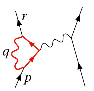
Figure 2. A diagram contributing to electron–electron scattering in QED. The loop has an ultraviolet divergence.

图2。量子电动力学中电子-电子散射的图解。这个环有一个紫外辐射。

The diagram in Figure 2 shows one of the several one-loop contributions to electron–electron scattering in QED. The electron on the left side of the diagram, represented by the solid line, starts out with 4-momentum p^μ and ends up with 4-momentum r^μ. It emits a virtual photon carrying r^μ − p^μ to transfer energy and momentum to the other electron. But in this diagram, before that happens, it emits another virtual photon carrying 4-momentum q^μ, and it reabsorbs this one after emitting the other virtual photon. Energy and momentum conservation do not determine the 4-momentum q^μ uniquely, so all possibilities contribute equally and we must integrate.

The diagram in Figure 2 shows one of the several one-loop contributions to electron–electron scattering in QED. The electron on the left side of the diagram, represented by the solid line, starts out with 4-momentum and ends up with 4-momentum . It emits a virtual photon carrying to transfer energy and momentum to the other electron. But in this diagram, before that happens, it emits another virtual photon carrying 4-momentum , and it reabsorbs this one after emitting the other virtual photon. Energy and momentum conservation do not determine the 4-momentum uniquely, so all possibilities contribute equally and we must integrate.

图2中的图式显示了量子电动力学中单圈对电子-电子散射的贡献之一。图左侧的电子，用实线表示，开始时是4动量的pμ，结束时是4动量的rμ。它发射一个携带rμ−pμ的虚光子，将能量和动量传递给另一个电子。但在这张图中，在这之前，它发射了另一个4动量的qμ的虚光子，它在发射了另一个虚光子后重新吸收了这个。能量和动量守恒并不能唯一地决定4动量qμ，所以所有的可能性都是相等的，我们必须积分。

This diagram's amplitude ends up with, among other things, a factor from the loop of

This diagram's amplitude ends up with, among other things, a factor from the loop of

除去其他因素，该图的振幅最终成为下圈的一个因子：

[math]\displaystyle{ -ie^3 \int \frac{d^4 q}{(2\pi)^4} \gamma^\mu \frac{i (\gamma^\alpha (r - q)_\alpha + m)}{(r - q)^2 - m^2 + i \epsilon} \gamma^\rho \frac{i (\gamma^\beta (p - q)_\beta + m)}{(p - q)^2 - m^2 + i \epsilon} \gamma^\nu \frac{-i g_{\mu\nu}}{q^2 + i\epsilon}. }[/math]

[math]\displaystyle{ -ie^3 \int \frac{d^4 q}{(2\pi)^4} \gamma^\mu \frac{i (\gamma^\alpha (r - q)_\alpha + m)}{(r - q)^2 - m^2 + i \epsilon} \gamma^\rho \frac{i (\gamma^\beta (p - q)_\beta + m)}{(p - q)^2 - m^2 + i \epsilon} \gamma^\nu \frac{-i g_{\mu\nu}}{q^2 + i\epsilon}. }[/math]

[math]\displaystyle{ -ie^3 \int \frac{d^4 q}{(2\pi)^4} \gamma^\mu \frac{i (\gamma^\alpha (r - q)_\alpha + m)}{(r - q)^2 - m^2 + i \epsilon} \gamma^\rho \frac{i (\gamma^\beta (p - q)_\beta + m)}{(p - q)^2 - m^2 + i \epsilon} \gamma^\nu \frac{-i g_{\mu\nu}}{q^2 + i\epsilon}. }[/math]

The various γ^μ factors in this expression are gamma matrices as in the covariant formulation of the Dirac equation; they have to do with the spin of the electron. The factors of e are the electric coupling constant, while the [math]\displaystyle{ i\epsilon }[/math] provide a heuristic definition of the contour of integration around the poles in the space of momenta. The important part for our purposes is the dependency on q^μ of the three big factors in the integrand, which are from the propagators of the two electron lines and the photon line in the loop.

The various factors in this expression are gamma matrices as in the covariant formulation of the Dirac equation; they have to do with the spin of the electron. The factors of are the electric coupling constant, while the [math]\displaystyle{ i\epsilon }[/math] provide a heuristic definition of the contour of integration around the poles in the space of momenta. The important part for our purposes is the dependency on of the three big factors in the integrand, which are from the propagators of the two electron lines and the photon line in the loop.

这个表达式中的各种γμ因子是和狄拉克方程的协变公式一样的伽马矩阵; 它们与电子的自旋有关。e的因子为电耦合常数，{\displaystyle i\epsilon}提供了动量空间中绕极点积分轮廓的启发式定义。对于我们的目的来说，重要的部分是被积函数中三个主要因子对qμ的依赖，这三个因子来自圈中的两条电子线和光子线的传播子。

This has a piece with two powers of q^μ on top that dominates at large values of q^μ (Pokorski 1987, p. 122):

This has a piece with two powers of on top that dominates at large values of (Pokorski 1987, p. 122):

这是一个上面有两个qμ的幂的部分，在较大的qμ值时占优势(Pokorski 1987, p. 122)：

[math]\displaystyle{ e^3 \gamma^\mu \gamma^\alpha \gamma^\rho \gamma^\beta \gamma_\mu \int \frac{d^4 q}{(2\pi)^4} \frac{q_\alpha q_\beta}{(r - q)^2 (p - q)^2 q^2}. }[/math]

[math]\displaystyle{ e^3 \gamma^\mu \gamma^\alpha \gamma^\rho \gamma^\beta \gamma_\mu \int \frac{d^4 q}{(2\pi)^4} \frac{q_\alpha q_\beta}{(r - q)^2 (p - q)^2 q^2}. }[/math]

[math]\displaystyle{ e^3 \gamma^\mu \gamma^\alpha \gamma^\rho \gamma^\beta \gamma_\mu \int \frac{d^4 q}{(2\pi)^4} \frac{q_\alpha q_\beta}{(r - q)^2 (p - q)^2 q^2}. }[/math]

This integral is divergent and infinite, unless we cut it off at finite energy and momentum in some way.

This integral is divergent and infinite, unless we cut it off at finite energy and momentum in some way.

这个积分是发散且无限的，除非我们在能量和动量有限的时候截断它。

Similar loop divergences occur in other quantum field theories.

Similar loop divergences occur in other quantum field theories.

类似的环散度也出现在其他量子场论中。

重整化的裸量

The solution was to realize that the quantities initially appearing in the theory's formulae (such as the formula for the Lagrangian), representing such things as the electron's electric charge and mass, as well as the normalizations of the quantum fields themselves, did not actually correspond to the physical constants measured in the laboratory. As written, they were bare quantities that did not take into account the contribution of virtual-particle loop effects to the physical constants themselves. Among other things, these effects would include the quantum counterpart of the electromagnetic back-reaction that so vexed classical theorists of electromagnetism. In general, these effects would be just as divergent as the amplitudes under consideration in the first place; so finite measured quantities would, in general, imply divergent bare quantities.

The solution was to realize that the quantities initially appearing in the theory's formulae (such as the formula for the Lagrangian), representing such things as the electron's electric charge and mass, as well as the normalizations of the quantum fields themselves, did not actually correspond to the physical constants measured in the laboratory. As written, they were bare quantities that did not take into account the contribution of virtual-particle loop effects to the physical constants themselves. Among other things, these effects would include the quantum counterpart of the electromagnetic back-reaction that so vexed classical theorists of electromagnetism. In general, these effects would be just as divergent as the amplitudes under consideration in the first place; so finite measured quantities would, in general, imply divergent bare quantities.

解决方案是认识到最初出现在理论公式中的量(比如拉格朗日公式) ，代表着电子的电荷和质量以及量子场本身的归一化，实际上并不符合在实验室测量所得的物理常数。如上所述，它们是裸量，并没有考虑虚粒子环效应对物理常数本身的影响。在其他情况中，这些影响还包括让经典电磁学理论家为难的电磁反作用量子对应物。一般来说，这些效应最初就会像考虑中的振幅一样发散; 所以有限的测量量通常意味着发散裸量。（OK）

To make contact with reality, then, the formulae would have to be rewritten in terms of measurable, renormalized quantities. The charge of the electron, say, would be defined in terms of a quantity measured at a specific kinematic renormalization point or subtraction point (which will generally have a characteristic energy, called the renormalization scale or simply the energy scale). The parts of the Lagrangian left over, involving the remaining portions of the bare quantities, could then be reinterpreted as counterterms, involved in divergent diagrams exactly canceling out the troublesome divergences for other diagrams.

To make contact with reality, then, the formulae would have to be rewritten in terms of measurable, renormalized quantities. The charge of the electron, say, would be defined in terms of a quantity measured at a specific kinematic renormalization point or subtraction point (which will generally have a characteristic energy, called the renormalization scale or simply the energy scale). The parts of the Lagrangian left over, involving the remaining portions of the bare quantities, could then be reinterpreted as counterterms, involved in divergent diagrams exactly canceling out the troublesome divergences for other diagrams.

因此，为了与现实接轨，这些公式必须以可测量的、重整化的量进行重写。例如，电子的电荷可以用在特定运动学重整化点或减点测量的量来定义(这种定义下通常具有一个特征能量，称为重整化标度或简称为能量标度)。剩下的涉及剩余裸量的拉格朗日部分，可以被重新解释为包含在发散图中，且正好抵消其他图发散现象的反项。（OK）

量子电动力学中的重整化

Figure 3. The vertex corresponding to the Z₁ counterterm cancels the divergence in Figure 2.

Figure 3. The vertex corresponding to the counterterm cancels the divergence in Figure 2.

图3。对应于反项的顶点抵消了图2中的发散。（OK）

For example, in the Lagrangian of QED

For example, in the Lagrangian of QED

例如，在量子电动力学的拉格朗日函数中（OK）

[math]\displaystyle{ \mathcal{L}=\bar\psi_B\left[i\gamma_\mu \left (\partial^\mu + ie_BA_B^\mu \right )-m_B\right]\psi_B -\frac{1}{4}F_{B\mu\nu}F_B^{\mu\nu} }[/math]

[math]\displaystyle{ \mathcal{L}=\bar\psi_B\left[i\gamma_\mu \left (\partial^\mu + ie_BA_B^\mu \right )-m_B\right]\psi_B -\frac{1}{4}F_{B\mu\nu}F_B^{\mu\nu} }[/math]

[math]\displaystyle{ \mathcal{L}=\bar\psi_B\left[i\gamma_\mu \left (\partial^\mu + ie_BA_B^\mu \right )-m_B\right]\psi_B -\frac{1}{4}F_{B\mu\nu}F_B^{\mu\nu} }[/math]

the fields and coupling constant are really bare quantities, hence the subscript B above. Conventionally the bare quantities are written so that the corresponding Lagrangian terms are multiples of the renormalized ones:

the fields and coupling constant are really bare quantities, hence the subscript above. Conventionally the bare quantities are written so that the corresponding Lagrangian terms are multiples of the renormalized ones:

磁场和耦合常数实际上是裸量（？），因此可见上面的下标如此B。通常，裸量相应的拉格朗日项是重整化项的倍数:

[math]\displaystyle{ \left(\bar\psi m \psi\right)_B = Z_0 \bar\psi m \psi }[/math]

[math]\displaystyle{ \left(\bar\psi m \psi\right)_B = Z_0 \bar\psi m \psi }[/math]

[math]\displaystyle{ \left(\bar\psi m \psi\right)_B = Z_0 \bar\psi m \psi }[/math]

[math]\displaystyle{ \left(\bar\psi\left(\partial^\mu + ieA^\mu \right )\psi\right)_B = Z_1 \bar\psi \left (\partial^\mu + ieA^\mu \right)\psi }[/math]

[math]\displaystyle{ \left(\bar\psi\left(\partial^\mu + ieA^\mu \right )\psi\right)_B = Z_1 \bar\psi \left (\partial^\mu + ieA^\mu \right)\psi }[/math]

[math]\displaystyle{ \left(\bar\psi\left(\partial^\mu + ieA^\mu \right )\psi\right)_B = Z_1 \bar\psi \left (\partial^\mu + ieA^\mu \right)\psi }[/math]

[math]\displaystyle{ \left(F_{\mu\nu}F^{\mu\nu}\right)_B = Z_3\, F_{\mu\nu}F^{\mu\nu}. }[/math]

[math]\displaystyle{ \left(F_{\mu\nu}F^{\mu\nu}\right)_B = Z_3\, F_{\mu\nu}F^{\mu\nu}. }[/math]

[math]\displaystyle{ \left(F_{\mu\nu}F^{\mu\nu}\right)_B = Z_3\, F_{\mu\nu}F^{\mu\nu}. }[/math]

Gauge invariance, via a Ward–Takahashi identity, turns out to imply that we can renormalize the two terms of the covariant derivative piece

Gauge invariance, via a Ward–Takahashi identity, turns out to imply that we can renormalize the two terms of the covariant derivative piece

通过 Ward-Takahashi 恒等式规范不变性，证明了我们可以重整共变导数的两个项在一起

[math]\displaystyle{ \bar \psi (\partial + ieA) \psi }[/math]

[math]\displaystyle{ \bar \psi (\partial + ieA) \psi }[/math]

[math]\displaystyle{ \bar \psi (\partial + ieA) \psi }[/math]

together (Pokorski 1987, p. 115), which is what happened to Z₂; it is the same as Z₁.

together (Pokorski 1987, p. 115), which is what happened to ; it is the same as .

(Pokorski 1987，第115页) ，这是实际上也是Z₂所发生的; 与Z₁相同。

A term in this Lagrangian, for example, the electron-photon interaction pictured in Figure 1, can then be written

A term in this Lagrangian, for example, the electron-photon interaction pictured in Figure 1, can then be written

拉格朗日函数中的一个项，例如图1所示的电子-光子相互作用，就可以被写出来

[math]\displaystyle{ \mathcal{L}_I = -e \bar\psi \gamma_\mu A^\mu \psi - (Z_1 - 1) e \bar\psi \gamma_\mu A^\mu \psi }[/math]

[math]\displaystyle{ \mathcal{L}_I = -e \bar\psi \gamma_\mu A^\mu \psi - (Z_1 - 1) e \bar\psi \gamma_\mu A^\mu \psi }[/math]

[math]\displaystyle{ \mathcal{L}_I = -e \bar\psi \gamma_\mu A^\mu \psi - (Z_1 - 1) e \bar\psi \gamma_\mu A^\mu \psi }[/math]

The physical constant e, the electron's charge, can then be defined in terms of some specific experiment: we set the renormalization scale equal to the energy characteristic of this experiment, and the first term gives the interaction we see in the laboratory (up to small, finite corrections from loop diagrams, providing such exotica as the high-order corrections to the magnetic moment). The rest is the counterterm. If the theory is renormalizable (see below for more on this), as it is in QED, the divergent parts of loop diagrams can all be decomposed into pieces with three or fewer legs, with an algebraic form that can be canceled out by the second term (or by the similar counterterms that come from Z₀ and Z₃).

The physical constant , the electron's charge, can then be defined in terms of some specific experiment: we set the renormalization scale equal to the energy characteristic of this experiment, and the first term gives the interaction we see in the laboratory (up to small, finite corrections from loop diagrams, providing such exotica as the high-order corrections to the magnetic moment). The rest is the counterterm. If the theory is renormalizable (see below for more on this), as it is in QED, the divergent parts of loop diagrams can all be decomposed into pieces with three or fewer legs, with an algebraic form that can be canceled out by the second term (or by the similar counterterms that come from and ).

这个物理常数，即电子的电荷，可以用一些特定的实验来定义: 我们把重整化标度设置为与这个实验的能量特征相等，第一个项就会给出我们在实验室中看到的相互作用(只要提供诸如磁矩的高阶修正，从环形图中就可以得到小的、有限的修正)。剩下的就是反项（？）了。如果理论是可重整化的(更多内容见下文) ，就像量子点动力学中一样，环路图的分叉部分都可以分解由成三个或更少分支（？）组成的部分，并且其拥有可以被第二项(或者类似的从Z₀得到的反项)抵消的代数形式。（OK）

The diagram with the Z₁ counterterm's interaction vertex placed as in Figure 3 cancels out the divergence from the loop in Figure 2.

The diagram with the counterterm's interaction vertex placed as in Figure 3 cancels out the divergence from the loop in Figure 2.

图3所示的反项的交互顶点Z₁的图抵消了图2中环的发散。

Historically, the splitting of the "bare terms" into the original terms and counterterms came before the renormalization group insight due to Kenneth Wilson. According to such renormalization group insights, detailed in the next section, this splitting is unnatural and actually unphysical, as all scales of the problem enter in continuous systematic ways.

Historically, the splitting of the "bare terms" into the original terms and counterterms came before the renormalization group insight due to Kenneth Wilson. According to such renormalization group insights, detailed in the next section, this splitting is unnatural and actually unphysical, as all scales of the problem enter in continuous systematic ways.

从历史上看，将“裸项”分解为原始项（？）和反项（？）的做法，早于肯尼思 · 威尔逊对重整化群的洞察。根据这些重整化群的洞察，在更细节的部分里这种分裂是非自然的也是非物理的，因为问题的所有尺度都是以连续的系统方式进入的（？）。

Running couplings

To minimize the contribution of loop diagrams to a given calculation (and therefore make it easier to extract results), one chooses a renormalization point close to the energies and momenta exchanged in the interaction. However, the renormalization point is not itself a physical quantity: the physical predictions of the theory, calculated to all orders, should in principle be independent of the choice of renormalization point, as long as it is within the domain of application of the theory. Changes in renormalization scale will simply affect how much of a result comes from Feynman diagrams without loops, and how much comes from the remaining finite parts of loop diagrams. One can exploit this fact to calculate the effective variation of physical constants with changes in scale. This variation is encoded by beta-functions, and the general theory of this kind of scale-dependence is known as the renormalization group.

To minimize the contribution of loop diagrams to a given calculation (and therefore make it easier to extract results), one chooses a renormalization point close to the energies and momenta exchanged in the interaction. However, the renormalization point is not itself a physical quantity: the physical predictions of the theory, calculated to all orders, should in principle be independent of the choice of renormalization point, as long as it is within the domain of application of the theory. Changes in renormalization scale will simply affect how much of a result comes from Feynman diagrams without loops, and how much comes from the remaining finite parts of loop diagrams. One can exploit this fact to calculate the effective variation of physical constants with changes in scale. This variation is encoded by beta-functions, and the general theory of this kind of scale-dependence is known as the renormalization group.

为了尽量减少环路图对给定计算的影响(从而使得计算结果更容易提取) ，可以选择一个接近相互作用中交换的能量和动量的重整化点。然而，重整化点本身并不是一个物理量: 在计算到所有的阶（？）之下，理论物理的预测，原则上应该独立于重整化点的选择，只要它在理论的应用范围内。重整化尺度的变化将影响无环费曼图产生的结果多少，以及来自环图剩余的有限部分的结果的多少。人们可以利用这一事实来计算物理常数随规模变化的有效变化。这种变化由 β 函数编码，这种尺度依赖的一般理论被称为重整化群。（OK）

Colloquially, particle physicists often speak of certain physical "constants" as varying with the energy of interaction, though in fact, it is the renormalization scale that is the independent quantity. This running does, however, provide a convenient means of describing changes in the behavior of a field theory under changes in the energies involved in an interaction. For example, since the coupling in quantum chromodynamics becomes small at large energy scales, the theory behaves more like a free theory as the energy exchanged in an interaction becomes large – a phenomenon known as asymptotic freedom. Choosing an increasing energy scale and using the renormalization group makes this clear from simple Feynman diagrams; were this not done, the prediction would be the same, but would arise from complicated high-order cancellations.

Colloquially, particle physicists often speak of certain physical "constants" as varying with the energy of interaction, though in fact, it is the renormalization scale that is the independent quantity. This running does, however, provide a convenient means of describing changes in the behavior of a field theory under changes in the energies involved in an interaction. For example, since the coupling in quantum chromodynamics becomes small at large energy scales, the theory behaves more like a free theory as the energy exchanged in an interaction becomes large – a phenomenon known as asymptotic freedom. Choosing an increasing energy scale and using the renormalization group makes this clear from simple Feynman diagrams; were this not done, the prediction would be the same, but would arise from complicated high-order cancellations.

通俗地说，粒子物理学家经常说的某些物理“常数”随着相互作用的能量而变化，尽管事实上，重整化标度才是独立量。然而，这种运行（？）确实提供了一种方便的手段来描述场理论在相互作用所涉及的能量变化下的行为变化。例如，由于量子色动力学中的耦合在大能量尺度下变小，该理论表现得更像一个自由理论（？），因为在相互作用中交换的能量变大了---- 这种现象被称为渐近自由（？）。选择一个递增的能量尺度并使用重整化群，可以从简单的费曼图中清楚地看出这一点; 如果不这样做，预测结果将是一样的，但是会出现复杂的高阶抵消。

For example,

For example,

比如说,

[math]\displaystyle{ I=\int_0^a \frac{1}{z}\,dz-\int_0^b \frac{1}{z}\,dz=\ln a-\ln b-\ln 0 +\ln 0 }[/math]

[math]\displaystyle{ I=\int_0^a \frac{1}{z}\,dz-\int_0^b \frac{1}{z}\,dz=\ln a-\ln b-\ln 0 +\ln 0 }[/math]

[math]\displaystyle{ I=\int_0^a \frac{1}{z}\,dz-\int_0^b \frac{1}{z}\,dz=\ln a-\ln b-\ln 0 +\ln 0 }[/math]

is ill-defined.

is ill-defined.

是不明确的。

To eliminate the divergence, simply change lower limit of integral into ε_a and ε_b:

To eliminate the divergence, simply change lower limit of integral into and :

为了去除发散，只需将积分的下限改为ε_a和ε_b:

[math]\displaystyle{ I=\ln a-\ln b-\ln{\varepsilon_a}+\ln{\varepsilon_b} = \ln \tfrac{a}{b} - \ln \tfrac{\varepsilon_a}{\varepsilon_b} }[/math]

[math]\displaystyle{ I=\ln a-\ln b-\ln{\varepsilon_a}+\ln{\varepsilon_b} = \ln \tfrac{a}{b} - \ln \tfrac{\varepsilon_a}{\varepsilon_b} }[/math]

[math]\displaystyle{ I=\ln a-\ln b-\ln{\varepsilon_a}+\ln{\varepsilon_b} = \ln \tfrac{a}{b} - \ln \tfrac{\varepsilon_a}{\varepsilon_b} }[/math]

Making sure 模板:Sfrac → 1, then I = ln 模板:Sfrac.

Making sure → 1}}, then ln .}}

确保模板:Sfrac → 1 ，然后 I = ln 模板:Sfrac.

正则化

Since the quantity ∞ − ∞ is ill-defined, in order to make this notion of canceling divergences precise, the divergences first have to be tamed mathematically using the theory of limits, in a process known as regularization (Weinberg, 1995).

Since the quantity is ill-defined, in order to make this notion of canceling divergences precise, the divergences first have to be tamed mathematically using the theory of limits, in a process known as regularization (Weinberg, 1995).

由于∞ − ∞的定义是不明确的，为了使散度抵消的概念更加精确，散度首先必须使用极限理论在数学上被驯服，这一过程被称为正则化(Weinberg, 1995)。

An essentially arbitrary modification to the loop integrands, or regulator, can make them drop off faster at high energies and momenta, in such a manner that the integrals converge. A regulator has a characteristic energy scale known as the cutoff; taking this cutoff to infinity (or, equivalently, the corresponding length/time scale to zero) recovers the original integrals.

An essentially arbitrary modification to the loop integrands, or regulator, can make them drop off faster at high energies and momenta, in such a manner that the integrals converge. A regulator has a characteristic energy scale known as the cutoff; taking this cutoff to infinity (or, equivalently, the corresponding length/time scale to zero) recovers the original integrals.

本质上任意修改圈被积函数，或调节器，可以使它们在高能量和动量下下降得更快，这样积分就会收敛。调节器有一个称为截止的特征能量标度；将这个截止值取为无穷大(或者，等价地，将相应的长度/时间标度取为零)，就可以恢复原来的积分。

With the regulator in place, and a finite value for the cutoff, divergent terms in the integrals then turn into finite but cutoff-dependent terms. After canceling out these terms with the contributions from cutoff-dependent counterterms, the cutoff is taken to infinity and finite physical results recovered. If physics on scales we can measure is independent of what happens at the very shortest distance and time scales, then it should be possible to get cutoff-independent results for calculations.

With the regulator in place, and a finite value for the cutoff, divergent terms in the integrals then turn into finite but cutoff-dependent terms. After canceling out these terms with the contributions from cutoff-dependent counterterms, the cutoff is taken to infinity and finite physical results recovered. If physics on scales we can measure is independent of what happens at the very shortest distance and time scales, then it should be possible to get cutoff-independent results for calculations.

有了调节器，并且截止值是有限的，积分中的发散项就变成了有限的，且与截止相关的项。在用依赖截止的反项抵消这些项后，截止到无穷大，并恢复有限的物理结果。如果我们可以测量的标度上的物理现象与在最短距离和时间尺度上发生的事情无关，那么就有可能得到与截止无关的计算结果。

Many different types of regulator are used in quantum field theory calculations, each with its advantages and disadvantages. One of the most popular in modern use is dimensional regularization, invented by Gerardus 't Hooft and Martinus J. G. Veltman, which tames the integrals by carrying them into a space with a fictitious fractional number of dimensions. Another is Pauli–Villars regularization, which adds fictitious particles to the theory with very large masses, such that loop integrands involving the massive particles cancel out the existing loops at large momenta.

Many different types of regulator are used in quantum field theory calculations, each with its advantages and disadvantages. One of the most popular in modern use is dimensional regularization, invented by Gerardus 't Hooft and Martinus J. G. Veltman, which tames the integrals by carrying them into a space with a fictitious fractional number of dimensions. Another is Pauli–Villars regularization, which adds fictitious particles to the theory with very large masses, such that loop integrands involving the massive particles cancel out the existing loops at large momenta.

量子场论计算中使用了许多不同类型的调节器，它们各有优缺点。在现代应用中最流行的是由Gerardus 't Hooft和Martinus J. G. Veltman发明的量纲正则化[21]，它通过将积分带入一个虚构的分数维数的空间来驯服积分。另一种是保利-维拉斯正则化，它以非常大的质量将虚构的粒子添加到理论中，这样涉及大质量粒子的圈积分在大动量中抵消了现有的圈。

Yet another regularization scheme is the lattice regularization, introduced by Kenneth Wilson, which pretends that hyper-cubical lattice constructs our space-time with fixed grid size. This size is a natural cutoff for the maximal momentum that a particle could possess when propagating on the lattice. And after doing a calculation on several lattices with different grid size, the physical result is extrapolated to grid size 0, or our natural universe. This presupposes the existence of a scaling limit.

Yet another regularization scheme is the lattice regularization, introduced by Kenneth Wilson, which pretends that hyper-cubical lattice constructs our space-time with fixed grid size. This size is a natural cutoff for the maximal momentum that a particle could possess when propagating on the lattice. And after doing a calculation on several lattices with different grid size, the physical result is extrapolated to grid size 0, or our natural universe. This presupposes the existence of a scaling limit.

另一种正则化方案是肯尼斯·威尔逊(Kenneth Wilson)提出的晶格正则化，它假设超立方晶格以固定的网格大小构建我们的时空。这一网格大小是粒子在晶格上传播时所能拥有的最大动量的自然截止。在对几个网格大小不同的网格进行计算后，物理结果外推到网格大小为0的情况，或是我们的自然宇宙。这以标度极限的存在为先决条件。

A rigorous mathematical approach to renormalization theory is the so-called causal perturbation theory, where ultraviolet divergences are avoided from the start in calculations by performing well-defined mathematical operations only within the framework of distribution theory. In this approach, divergences are replaced by ambiguity: corresponding to a divergent diagram is a term which now has a finite, but undetermined, coefficient. Other principles, such as gauge symmetry, must then be used to reduce or eliminate the ambiguity.

A rigorous mathematical approach to renormalization theory is the so-called causal perturbation theory, where ultraviolet divergences are avoided from the start in calculations by performing well-defined mathematical operations only within the framework of distribution theory. In this approach, divergences are replaced by ambiguity: corresponding to a divergent diagram is a term which now has a finite, but undetermined, coefficient. Other principles, such as gauge symmetry, must then be used to reduce or eliminate the ambiguity.

重正化理论的一个严格的数学方法是因果摄动理论，其中紫外散度从计算的开始就可以避免，只需要在分布理论的框架内进行定义良好的数学运算。在这种方法中，散度可以由模糊度代替：这个对应于散度图的术语是一个有限的，但未确定的系数。之后其他原理，如规范对称，必须用来减少或消除模糊度。

Zeta函数正则化

Julian Schwinger discovered a relationship between zeta function regularization and renormalization, using the asymptotic relation:

Julian Schwinger discovered a relationship between zeta function regularization and renormalization, using the asymptotic relation:

朱利安·施温格使用渐近关系作为调节器（其中Λ → ∞）：

[math]\displaystyle{ I(n, \Lambda )= \int_0^{\Lambda }dp\,p^n \sim 1+2^n+3^n+\cdots+ \Lambda^n \to \zeta(-n) }[/math]

[math]\displaystyle{ I(n, \Lambda )= \int_0^{\Lambda }dp\,p^n \sim 1+2^n+3^n+\cdots+ \Lambda^n \to \zeta(-n) }[/math]

[math]\displaystyle{ I(n, \Lambda )= \int_0^{\Lambda }dp\,p^n \sim 1+2^n+3^n+\cdots+ \Lambda^n \to \zeta(-n) }[/math]

as the regulator Λ → ∞. Based on this, he considered using the values of ζ(−n) to get finite results. Although he reached inconsistent results, an improved formula studied by Hartle, J. Garcia, and based on the works by E. Elizalde includes the technique of the zeta regularization algorithm

as the regulator . Based on this, he considered using the values of to get finite results. Although he reached inconsistent results, an improved formula studied by Hartle, J. Garcia, and based on the works by E. Elizalde includes the technique of the zeta regularization algorithm

发现了Zeta函数正则化重整化之间的联系。在此基础上，他考虑利用ζ(−n)的值来得到有限的结果。尽管他得出的结果不一致，但是由Hartle, J. Garcia研究的改进公式，并基于E. Elizalde的工作，依然囊括了zeta正则化算法的技术

[math]\displaystyle{ I(n, \Lambda) = \frac{n}{2}I(n-1, \Lambda) + \zeta(-n) - \sum_{r=1}^{\infty}\frac{B_{2r}}{(2r)!} a_{n,r}(n-2r+1) I(n-2r, \Lambda), }[/math]

[math]\displaystyle{ I(n, \Lambda) = \frac{n}{2}I(n-1, \Lambda) + \zeta(-n) - \sum_{r=1}^{\infty}\frac{B_{2r}}{(2r)!} a_{n,r}(n-2r+1) I(n-2r, \Lambda), }[/math]

[math]\displaystyle{ I(n, \Lambda) = \frac{n}{2}I(n-1, \Lambda) + \zeta(-n) - \sum_{r=1}^{\infty}\frac{B_{2r}}{(2r)!} a_{n,r}(n-2r+1) I(n-2r, \Lambda), }[/math]

where the B's are the Bernoulli numbers and

where the Bs are the Bernoulli numbers and

其中B代表伯努利数，并且

[math]\displaystyle{ a_{n,r}= \frac{\Gamma(n+1)}{\Gamma(n-2r+2)}. }[/math]

[math]\displaystyle{ a_{n,r}= \frac{\Gamma(n+1)}{\Gamma(n-2r+2)}. }[/math]

[math]\displaystyle{ a_{n,r}= \frac{\Gamma(n+1)}{\Gamma(n-2r+2)}. }[/math]

So every I(m, Λ) can be written as a linear combination of ζ(−1), ζ(−3), ζ(−5), ..., ζ(−m).

So every can be written as a linear combination of .

所以每个I(m, Λ)都可以写成ζ(−1), ζ(−3), ζ(−5), ..., ζ(−m)。

Or simply using Abel–Plana formula we have for every divergent integral:

Or simply using Abel–Plana formula we have for every divergent integral:

或者简单地对每一个发散积分使用阿贝尔-普拉纳公式：

[math]\displaystyle{ \zeta(-m, \beta )-\frac{\beta ^{m}}{2}-i\int_ 0 ^{\infty}dt \frac{ (it+\beta)^{m}-(-it+\beta)^{m}}{e^{2 \pi t}-1}=\int_0^\infty dp \, (p+\beta)^m }[/math]

[math]\displaystyle{ \zeta(-m, \beta )-\frac{\beta ^{m}}{2}-i\int_ 0 ^{\infty}dt \frac{ (it+\beta)^{m}-(-it+\beta)^{m}}{e^{2 \pi t}-1}=\int_0^\infty dp \, (p+\beta)^m }[/math]

[math]\displaystyle{ \zeta(-m, \beta )-\frac{\beta ^{m}}{2}-i\int_ 0 ^{\infty}dt \frac{ (it+\beta)^{m}-(-it+\beta)^{m}}{e^{2 \pi t}-1}=\int_0^\infty dp \, (p+\beta)^m }[/math]

valid when m > 0, Here the zeta function is Hurwitz zeta function and Beta is a positive real number.

valid when , Here the zeta function is Hurwitz zeta function and Beta is a positive real number.

当m>0时成立，这里的Zeta函数是赫尔维茨函数，其中β是一个正实数。

The "geometric" analogy is given by, (if we use rectangle method) to evaluate the integral so:

The "geometric" analogy is given by, (if we use rectangle method) to evaluate the integral so:

“几何”的类比由下式给出，(如果我们使用矩形法)来计算积分：

[math]\displaystyle{ \int_0^\infty dx \, (\beta +x)^m \approx \sum_{n=0}^\infty h^{m+1} \zeta \left( \beta h^{-1} , -m \right) }[/math]

[math]\displaystyle{ \int_0^\infty dx \, (\beta +x)^m \approx \sum_{n=0}^\infty h^{m+1} \zeta \left( \beta h^{-1} , -m \right) }[/math]

[math]\displaystyle{ \int_0^\infty dx \, (\beta +x)^m \approx \sum_{n=0}^\infty h^{m+1} \zeta \left( \beta h^{-1} , -m \right) }[/math]

Using Hurwitz zeta regularization plus the rectangle method with step h (not to be confused with Planck's constant).

Using Hurwitz zeta regularization plus the rectangle method with step h (not to be confused with Planck's constant).

使用赫尔维茨Zeta正则化加上步骤h的矩形法(此处h不要与普朗克常数混淆)。

The logarithmic divergent integral has the regularization

The logarithmic divergent integral has the regularization

对数发散积分具有正则化

[math]\displaystyle{ \sum_{n=0}^{\infty} \frac{1}{n+a}= - \psi (a)+\log (a) }[/math]

[math]\displaystyle{ \sum_{n=0}^{\infty} \frac{1}{n+a}= - \psi (a)+\log (a) }[/math]

[math]\displaystyle{ \sum_{n=0}^{\infty} \frac{1}{n+a}= - \psi (a)+\log (a) }[/math]

since for the Harmonic series [math]\displaystyle{ \sum_{n=0}^{\infty} \frac{1}{an+1} }[/math] in the limit [math]\displaystyle{ a \to 0 }[/math] we must recover the series [math]\displaystyle{ \sum_{n=0}^{\infty}1 =1/2 }[/math]

since for the Harmonic series [math]\displaystyle{ \sum_{n=0}^{\infty} \frac{1}{an+1} }[/math] in the limit [math]\displaystyle{ a \to 0 }[/math] we must recover the series [math]\displaystyle{ \sum_{n=0}^{\infty}1 =1/2 }[/math]

因为对于调和级数[math]\displaystyle{ \sum_{n=0}^{\infty} \frac{1}{an+1} }[/math]在a趋近于零处，我们必须恢复级数[math]\displaystyle{ \sum_{n=0}^{\infty}1 =1/2 }[/math]

For multi-loop integrals that will depend on several variables [math]\displaystyle{ k_1, \cdots, k_n }[/math] we can make a change of variables to polar coordinates and then replace the integral over the angles [math]\displaystyle{ \int d \Omega }[/math] by a sum so we have only a divergent integral, that will depend on the modulus [math]\displaystyle{ r^2 = k_1^2 +\cdots+k_n^2 }[/math] and then we can apply the zeta regularization algorithm, the main idea for multi-loop integrals is to replace the factor [math]\displaystyle{ F(q_1,\cdots,q_n) }[/math] after a change to hyperspherical coordinates F(r, Ω) so the UV overlapping divergences are encoded in variable r. In order to regularize these integrals one needs a regulator, for the case of multi-loop integrals, these regulator can be taken as

For multi-loop integrals that will depend on several variables [math]\displaystyle{ k_1, \cdots, k_n }[/math] we can make a change of variables to polar coordinates and then replace the integral over the angles [math]\displaystyle{ \int d \Omega }[/math] by a sum so we have only a divergent integral, that will depend on the modulus [math]\displaystyle{ r^2 = k_1^2 +\cdots+k_n^2 }[/math] and then we can apply the zeta regularization algorithm, the main idea for multi-loop integrals is to replace the factor [math]\displaystyle{ F(q_1,\cdots,q_n) }[/math] after a change to hyperspherical coordinates so the UV overlapping divergences are encoded in variable . In order to regularize these integrals one needs a regulator, for the case of multi-loop integrals, these regulator can be taken as

对于依赖于多个变量[math]\displaystyle{ k_1, \cdots, k_n }[/math]的多圈积分，我们可以将变量转换为极坐标，然后用一个和替换角度上的积分[math]\displaystyle{ \int d \Omega }[/math]，因此我们只有一个发散积分，它取决于模[math]\displaystyle{ r^2 = k_1^2 +\cdots+k_n^2 }[/math]，然后我们可以应用Zeta正则化算法，多圈积分的主要思想是将因子[math]\displaystyle{ F(q_1,\cdots,q_n) }[/math]替换为超球坐标F(r, Ω)，使紫外重叠散度编码在变量r中。为了正则化这些积分，需要一个调节器，对于多圈积分的情况，这些调节器可以被视为：

[math]\displaystyle{ \left (1+ \sqrt{q}_{i}q^{i} \right )^{-s} }[/math]

[math]\displaystyle{ \left (1+ \sqrt{q}_{i}q^{i} \right )^{-s} }[/math]

[math]\displaystyle{ \left (1+ \sqrt{q}_{i}q^{i} \right )^{-s} }[/math]

so the multi-loop integral will converge for big enough s using the Zeta regularization we can analytic continue the variable s to the physical limit where s = 0 and then regularize any UV integral, by replacing a divergent integral by a linear combination of divergent series, which can be regularized in terms of the negative values of the Riemann zeta function ζ(−m).

so the multi-loop integral will converge for big enough using the Zeta regularization we can analytic continue the variable to the physical limit where 0}} and then regularize any UV integral, by replacing a divergent integral by a linear combination of divergent series, which can be regularized in terms of the negative values of the Riemann zeta function .

所以多圈积分在足够大的s时收敛，使用正则化我们可以继续分析变量s直到s = 0的物理极限，然后正则化任何紫外积分，通过用发散级数的线性组合替换发散积分，它可以正则化为黎曼ζ函数的负值ζ(−m)。

态度以及解读

The early formulators of QED and other quantum field theories were, as a rule, dissatisfied with this state of affairs. It seemed illegitimate to do something tantamount to subtracting infinities from infinities to get finite answers.

The early formulators of QED and other quantum field theories were, as a rule, dissatisfied with this state of affairs. It seemed illegitimate to do something tantamount to subtracting infinities from infinities to get finite answers.

量子电动力学和其他量子场论的早期规范者通常对这种（重整化的）处理方式不满意。为了得到有限的答案而从无限中减去无限，这似乎是不合理的。

Freeman Dyson argued that these infinities are of a basic nature and cannot be eliminated by any formal mathematical procedures, such as the renormalization method.

Freeman Dyson argued that these infinities are of a basic nature and cannot be eliminated by any formal mathematical procedures, such as the renormalization method.

弗里曼戴森认为，这些无穷大是一个自然的基本性质，不能被任何形式的数学程序所消除，比如重整化方法。

Dirac's criticism was the most persistent. As late as 1975, he was saying:

Dirac's criticism was the most persistent. As late as 1975, he was saying:

狄拉克的批评是最持久的。直到1975年，他仍表示:

Most physicists are very satisfied with the situation. They say: 'Quantum electrodynamics is a good theory and we do not have to worry about it any more.' I must say that I am very dissatisfied with the situation because this so-called 'good theory' does involve neglecting infinities which appear in its equations, ignoring them in an arbitrary way. This is just not sensible mathematics. Sensible mathematics involves disregarding a quantity when it is small – not neglecting it just because it is infinitely great and you do not want it!

Most physicists are very satisfied with the situation. They say: 'Quantum electrodynamics is a good theory and we do not have to worry about it any more.' I must say that I am very dissatisfied with the situation because this so-called 'good theory' does involve neglecting infinities which appear in its equations, ignoring them in an arbitrary way. This is just not sensible mathematics. Sensible mathematics involves disregarding a quantity when it is small – not neglecting it just because it is infinitely great and you do not want it!

大多数物理学家对这种情况非常满意。他们说: ‘量子电动力学理论是一个很好的理论，我们再也不用担心它了’。但我必须说，我对这种情况非常不满意，因为这种所谓的“好理论”确实有涉及忽视方程式中出现的无穷大，且以一种武断的方式忽视它们。这根本不是合理的数学。合理的数学涉及对微小量的忽略，而不是仅仅因为一个量无限大，你不想要它就可以忽略它！

Another important critic was Feynman. Despite his crucial role in the development of quantum electrodynamics, he wrote the following in 1985:

Another important critic was Feynman. Despite his crucial role in the development of quantum electrodynamics, he wrote the following in 1985:

另一位重要的评论家是费曼。尽管他在量子电动力学的发展中扮演了关键角色，他在1985年写道:

The shell game that we play is technically called 'renormalization'. But no matter how clever the word, it is still what I would call a dippy process! Having to resort to such hocus-pocus has prevented us from proving that the theory of quantum electrodynamics is mathematically self-consistent. It's surprising that the theory still hasn't been proved self-consistent one way or the other by now; I suspect that renormalization is not mathematically legitimate.

The shell game that we play is technically called 'renormalization'. But no matter how clever the word, it is still what I would call a dippy process! Having to resort to such hocus-pocus has prevented us from proving that the theory of quantum electrodynamics is mathematically self-consistent. It's surprising that the theory still hasn't been proved self-consistent one way or the other by now; I suspect that renormalization is not mathematically legitimate.

我们玩的这个骗局在技术上叫做“重整化”。但是不管这个词多么聪明，它仍然是我所说的一个含糊的过程！不得不求助于这样的骗术阻碍了我们证明量子电动力学理论在数学上是自洽的脚步。令人惊讶的是，到目前为止，这个理论仍然没有以这样或那样的方式被证明是自洽的; 我怀疑重整化在数学上是不正当的。

Feynman was concerned that all field theories known in the 1960s had the property that the interactions become infinitely strong at short enough distance scales. This property called a Landau pole, made it plausible that quantum field theories were all inconsistent. In 1974, Gross, Politzer and Wilczek showed that another quantum field theory, quantum chromodynamics, does not have a Landau pole. Feynman, along with most others, accepted that QCD was a fully consistent theory.

Feynman was concerned that all field theories known in the 1960s had the property that the interactions become infinitely strong at short enough distance scales. This property called a Landau pole, made it plausible that quantum field theories were all inconsistent. In 1974, Gross, Politzer and Wilczek showed that another quantum field theory, quantum chromodynamics, does not have a Landau pole. Feynman, along with most others, accepted that QCD was a fully consistent theory.

费曼担心，在20世纪60年代所有已知的场理论都有这样的特性: 在足够短的距离尺度上，相互作用会变得无限强。这个性质被称为Landau pole，它使量子场理论完全不一致的说法变得可信。1974年，Gross，Politzer 和 Wilczek 证明了另一个量子场论（即量子色动力学），并没有Landau pole。费曼和其他大多数人一样，承认量子色动力学是一个完全一致的理论。

The general unease was almost universal in texts up to the 1970s and 1980s. Beginning in the 1970s, however, inspired by work on the renormalization group and effective field theory, and despite the fact that Dirac and various others—all of whom belonged to the older generation—never withdrew their criticisms, attitudes began to change, especially among younger theorists. Kenneth G. Wilson and others demonstrated that the renormalization group is useful in statistical field theory applied to condensed matter physics, where it provides important insights into the behavior of phase transitions. In condensed matter physics, a physical short-distance regulator exists: matter ceases to be continuous on the scale of atoms. Short-distance divergences in condensed matter physics do not present a philosophical problem since the field theory is only an effective, smoothed-out representation of the behavior of matter anyway; there are no infinities since the cutoff is always finite, and it makes perfect sense that the bare quantities are cutoff-dependent.

The general unease was almost universal in texts up to the 1970s and 1980s. Beginning in the 1970s, however, inspired by work on the renormalization group and effective field theory, and despite the fact that Dirac and various others—all of whom belonged to the older generation—never withdrew their criticisms, attitudes began to change, especially among younger theorists. Kenneth G. Wilson and others demonstrated that the renormalization group is useful in statistical field theory applied to condensed matter physics, where it provides important insights into the behavior of phase transitions. In condensed matter physics, a physical short-distance regulator exists: matter ceases to be continuous on the scale of atoms. Short-distance divergences in condensed matter physics do not present a philosophical problem since the field theory is only an effective, smoothed-out representation of the behavior of matter anyway; there are no infinities since the cutoff is always finite, and it makes perfect sense that the bare quantities are cutoff-dependent.

直到20世纪70年代和80年代，这种普遍的不安在文献中几乎是普遍存在的。然而，从20世纪70年代开始，尽管狄拉克和其他各种人---- 那些老一辈的理论家---- 从未收回他们的批评，受到重整化群理论和有效场理论工作的启发，人们的态度开始改变，尤其是在年轻的理论家中。肯尼斯·威尔森和其他人证明了重整化群对凝聚态物理学中统计场理论的应用有帮助，因为它对相变行为提供了重要的见解。在凝聚态物理学，存在一个物理的短距离调节器:在原子规模下，物质不再是连续的。凝聚态物理学中的短距离发散并不构成哲学问题，因为场论实际也只是对物质行为的一种有效的、平滑的理想表示; 因为截止值总是有限的，所以没有无限性，而且裸量依赖于截止值也是完全合理的。

If QFT holds all the way down past the Planck length (where it might yield to string theory, causal set theory or something different), then there may be no real problem with short-distance divergences in particle physics either; all field theories could simply be effective field theories. In a sense, this approach echoes the older attitude that the divergences in QFT speak of human ignorance about the workings of nature, but also acknowledges that this ignorance can be quantified and that the resulting effective theories remain useful.

If QFT holds all the way down past the Planck length (where it might yield to string theory, causal set theory or something different), then there may be no real problem with short-distance divergences in particle physics either; all field theories could simply be effective field theories. In a sense, this approach echoes the older attitude that the divergences in QFT speak of human ignorance about the workings of nature, but also acknowledges that this ignorance can be quantified and that the resulting effective theories remain useful.

如果量子场论能一直保持成立到普朗克长度以下(在那里它可能会产生弦论、因果集合论或其他不同的理论) ，那么粒子物理学中的短距离发散可能也不存在实质的问题; 所有场论都可能是有效场论。在某种意义上，这种方法呼应了以前的态度，即量子力学中的发散说明了人类对自然运作规律的无知，但也承认这种无知是可以量化的，且由此产生的有效理论仍然是有用的。

Be that as it may, Salam's remark in 1972 seems still relevant

Be that as it may, Salam's remark in 1972 seems still relevant

尽管如此，萨拉姆在1972年的言论似乎仍然有意义

Field-theoretic infinities — first encountered in Lorentz's computation of electron self-mass — have persisted in classical electrodynamics for seventy and in quantum electrodynamics for some thirty-five years. These long years of frustration have left in the subject a curious affection for the infinities and a passionate belief that they are an inevitable part of nature; so much so that even the suggestion of a hope that they may, after all, be circumvented — and finite values for the renormalization constants computed — is considered irrational. Compare Russell's postscript to the third volume of his autobiography The Final Years, 1944–1969 (George Allen and Unwin, Ltd., London 1969), p. 221:

Field-theoretic infinities — first encountered in Lorentz's computation of electron self-mass — have persisted in classical electrodynamics for seventy and in quantum electrodynamics for some thirty-five years. These long years of frustration have left in the subject a curious affection for the infinities and a passionate belief that they are an inevitable part of nature; so much so that even the suggestion of a hope that they may, after all, be circumvented — and finite values for the renormalization constants computed — is considered irrational. Compare Russell's postscript to the third volume of his autobiography  The Final Years, 1944–1969 (George Allen and Unwin, Ltd., London 1969), p. 221:

场论的无穷大首次出现在洛伦兹对电子自质量的计算过程中，它在经典电动力学中已经存在了七十年，在量子电动力学中也已存在了35年。这么多年的挫折使得研究这个课题的人对无穷大产生了一种奇怪的感情，并且热切地相信它们是自然界不可避免的一部分; 以至于即使他们有可能避开了正解，有限的重整化常数可被计算--这样的希望都被认为是不合理的。将罗素的附言与他的自传《最后的岁月，1944-1969》(乔治 · 艾伦和安文出版社，伦敦，1969年)的第三卷相比较，于第221页:

In the modern world, if communities are unhappy, it is often because they have ignorances, habits, beliefs, and passions, which are dearer to them than happiness or even life. I find many men in our dangerous age who seem to be in love with misery and death, and who grow angry when hopes are suggested to them. They think hope is irrational and that, in sitting down to lazy despair, they are merely facing facts.

In the modern world, if communities are unhappy, it is often because they have ignorances, habits, beliefs, and passions, which are dearer to them than happiness or even life. I find many men in our dangerous age who seem to be in love with misery and death, and who grow angry when hopes are suggested to them. They think hope is irrational and that, in sitting down to lazy despair, they are merely facing facts.

在现代社会，如果团体不幸福，那往往是因为他们有那些比幸福甚至生命更重要的无知、习惯、信仰和激情。我发现在我们这个危险的时代，有许多人似乎爱上了痛苦和死亡，以至于当面对希望时，他们会生气起来。他们认为希望是非理性的，坐下来懒洋洋地绝望只是在面对事实而已（？）。

In QFT, the value of a physical constant, in general, depends on the scale that one chooses as the renormalization point, and it becomes very interesting to examine the renormalization group running of physical constants under changes in the energy scale. The coupling constants in the Standard Model of particle physics vary in different ways with increasing energy scale: the coupling of quantum chromodynamics and the weak isospin coupling of the electroweak force tend to decrease, and the weak hypercharge coupling of the electroweak force tends to increase. At the colossal energy scale of 10¹⁵ GeV (far beyond the reach of our current particle accelerators), they all become approximately the same size (Grotz and Klapdor 1990, p. 254), a major motivation for speculations about grand unified theory. Instead of being only a worrisome problem, renormalization has become an important theoretical tool for studying the behavior of field theories in different regimes.

In QFT, the value of a physical constant, in general, depends on the scale that one chooses as the renormalization point, and it becomes very interesting to examine the renormalization group running of physical constants under changes in the energy scale. The coupling constants in the Standard Model of particle physics vary in different ways with increasing energy scale: the coupling of quantum chromodynamics and the weak isospin coupling of the electroweak force tend to decrease, and the weak hypercharge coupling of the electroweak force tends to increase. At the colossal energy scale of 10¹⁵ GeV (far beyond the reach of our current particle accelerators), they all become approximately the same size (Grotz and Klapdor 1990, p. 254), a major motivation for speculations about grand unified theory. Instead of being only a worrisome problem, renormalization has become an important theoretical tool for studying the behavior of field theories in different regimes.

在量子场论中，一个物理常数的值，一般来说，取决于我们选择的重整化点的尺度，在能量尺度变化的情况下，研究重整化群物理常数的运行变得非常有趣。粒子物理标准模型中的耦合常数随着能量的增加而以不同的方式变化: 量子色动力学的耦合和电弱力的弱同位旋耦合趋于减小，电弱力的弱超荷耦合趋于增加。在10¹⁵ GeV 的巨大能量尺度内(远远超出我们现有的粒子加速器的能量范围) ，它们都变得大致相同(Grotz 和 Klapdor 1990，p. 254) ，这是推测大统一理论的主要动机。重整化已经不再是一个令人担忧的问题，而是成为研究不同区域中场理论行为的一个重要理论工具。

If a theory featuring renormalization (e.g. QED) can only be sensibly interpreted as an effective field theory, i.e. as an approximation reflecting human ignorance about the workings of nature, then the problem remains of discovering a more accurate theory that does not have these renormalization problems. As Lewis Ryder has put it, "In the Quantum Theory, these [classical] divergences do not disappear; on the contrary, they appear to get worse. And despite the comparative success of renormalisation theory, the feeling remains that there ought to be a more satisfactory way of doing things."

If a theory featuring renormalization (e.g. QED) can only be sensibly interpreted as an effective field theory, i.e. as an approximation reflecting human ignorance about the workings of nature, then the problem remains of discovering a more accurate theory that does not have these renormalization problems. As Lewis Ryder has put it, "In the Quantum Theory, these [classical] divergences do not disappear; on the contrary, they appear to get worse. And despite the comparative success of renormalisation theory, the feeling remains that there ought to be a more satisfactory way of doing things."

如果一个具有重整化特征的理论(例如:量子电动力学(QED))只能合理地被解释为一种有效场理论，即作为反映人类对自然规律的无知的近似反应，那么问题仍在于发现一个更精确的，不存在这些重整化问题的理论。正如路易斯 · 莱德所说，“在量子理论中，这些[经典]发散并没有消失; 相反，它们似乎变得更糟。尽管重整化理论相对成功，但人们仍然认为，应该有一种更令人满意的处理方法。”

可重整性

From this philosophical reassessment, a new concept follows naturally: the notion of renormalizability. Not all theories lend themselves to renormalization in the manner described above, with a finite supply of counterterms and all quantities becoming cutoff-independent at the end of the calculation. If the Lagrangian contains combinations of field operators of high enough dimension in energy units, the counterterms required to cancel all divergences proliferate to infinite number, and, at first glance, the theory would seem to gain an infinite number of free parameters and therefore lose all predictive power, becoming scientifically worthless. Such theories are called nonrenormalizable.

From this philosophical reassessment, a new concept follows naturally: the notion of renormalizability. Not all theories lend themselves to renormalization in the manner described above, with a finite supply of counterterms and all quantities becoming cutoff-independent at the end of the calculation. If the Lagrangian contains combinations of field operators of high enough dimension in energy units, the counterterms required to cancel all divergences proliferate to infinite number, and, at first glance, the theory would seem to gain an infinite number of free parameters and therefore lose all predictive power, becoming scientifically worthless. Such theories are called nonrenormalizable.

从这一哲学的重新评价中，一个新的概念自然地产生了：即可重整性。不是所有的理论都能以上述的方式重整化，且在计算结束时，有限的反项和所有的量变得截止无关。如果拉格朗日算子包含能量单位足够高维的场算符组合，抵消所有散度所需要的反项激增到无穷多个。乍一看这个理论似乎获得了无数的自由参数，然而却因此失去了所有的预测能力，也就在科学上变得毫无价值。这样的理论被称为不可重整的理论。

The Standard Model of particle physics contains only renormalizable operators, but the interactions of general relativity become nonrenormalizable operators if one attempts to construct a field theory of quantum gravity in the most straightforward manner (treating the metric in the Einstein–Hilbert Lagrangian as a perturbation about the Minkowski metric), suggesting that perturbation theory is useless in application to quantum gravity.

The Standard Model of particle physics contains only renormalizable operators, but the interactions of general relativity become nonrenormalizable operators if one attempts to construct a field theory of quantum gravity in the most straightforward manner (treating the metric in the Einstein–Hilbert Lagrangian as a perturbation about the Minkowski metric), suggesting that perturbation theory is useless in application to quantum gravity.

粒子物理的标准模型只包含可重整算子，但如果有人试图以最直接的方式构建量子引力场理论(将爱因斯坦-希尔伯特拉格朗日公式中的度规视为对闵可夫斯基度规的扰动)，广义相对论的相互作用就会成为不可重整化的算子，这表明微扰理论在量子引力中的应用并不令人满意。

However, in an effective field theory, "renormalizability" is, strictly speaking, a misnomer. In nonrenormalizable effective field theory, terms in the Lagrangian do multiply to infinity, but have coefficients suppressed by ever-more-extreme inverse powers of the energy cutoff. If the cutoff is a real, physical quantity—that is, if the theory is only an effective description of physics up to some maximum energy or minimum distance scale—then these additional terms could represent real physical interactions. Assuming that the dimensionless constants in the theory do not get too large, one can group calculations by inverse powers of the cutoff, and extract approximate predictions to finite order in the cutoff that still have a finite number of free parameters. It can even be useful to renormalize these "nonrenormalizable" interactions.

However, in an effective field theory, "renormalizability" is, strictly speaking, a misnomer. In nonrenormalizable effective field theory, terms in the Lagrangian do multiply to infinity, but have coefficients suppressed by ever-more-extreme inverse powers of the energy cutoff. If the cutoff is a real, physical quantity—that is, if the theory is only an effective description of physics up to some maximum energy or minimum distance scale—then these additional terms could represent real physical interactions. Assuming that the dimensionless constants in the theory do not get too large, one can group calculations by inverse powers of the cutoff, and extract approximate predictions to finite order in the cutoff that still have a finite number of free parameters. It can even be useful to renormalize these "nonrenormalizable" interactions.

然而，在有效场理论中，严格来说，“重整化性”是一个误称。在非重整有效场理论中，拉格朗日算子的各项确实可以增加到无穷，但系数会被越来越极端的能量截止逆幂所抑制。如果截止是一个真实的物理量，也就是说，如果这个理论仅仅是对某些最大能量或最小距离尺度下的物理的有效描述，那么这些额外的项就可以代表真实的物理相互作用。假设理论中的无量纲常数不会变得太大，我们可以通过截止的逆幂来分组计算，在包含有限数量自由参数的截止中提取有限阶的近似预测。甚至可以对这些“不可重整化”的交互进行重整化。

Nonrenormalizable interactions in effective field theories rapidly become weaker as the energy scale becomes much smaller than the cutoff. The classic example is the Fermi theory of the weak nuclear force, a nonrenormalizable effective theory whose cutoff is comparable to the mass of the W particle. This fact may also provide a possible explanation for why almost all of the particle interactions we see are describable by renormalizable theories. It may be that any others that may exist at the GUT or Planck scale simply become too weak to detect in the realm we can observe, with one exception: gravity, whose exceedingly weak interaction is magnified by the presence of the enormous masses of stars and planets.

Nonrenormalizable interactions in effective field theories rapidly become weaker as the energy scale becomes much smaller than the cutoff. The classic example is the Fermi theory of the weak nuclear force, a nonrenormalizable effective theory whose cutoff is comparable to the mass of the W particle. This fact may also provide a possible explanation for why almost all of the particle interactions we see are describable by renormalizable theories. It may be that any others that may exist at the GUT or Planck scale simply become too weak to detect in the realm we can observe, with one exception: gravity, whose exceedingly weak interaction is magnified by the presence of the enormous masses of stars and planets.

在有效场论中，当能量尺度比截止小得多时，非重整相互作用迅速变弱。经典例子是弱核力的费米理论，这是一种非重整有效理论，其截止可与W粒子的质量相当。这一事实也提供了一种可能的解释—为什么我们看到几乎所有粒子相互作用都可以用重整化理论来描述。可能存在于统一场论或普朗克尺度上的任何其他物质在我们能观测到的领域中都变得太弱了。只有一个例外：引力，它极其微弱的相互作用被巨大质量的恒星和行星的存在放大了。

重整化方案

In actual calculations, the counterterms introduced to cancel the divergences in Feynman diagram calculations beyond tree level must be fixed using a set of renormalisation conditions. The common renormalization schemes in use include:

In actual calculations, the counterterms introduced to cancel the divergences in Feynman diagram calculations beyond tree level must be fixed using a set of renormalisation conditions. The common renormalization schemes in use include:

在实际计算中，为了抵消费曼图计算中超出树图的散度而引入的反项必须使用一组重整化条件来解决。常用的重整化方案包括：

• Minimal subtraction (MS) scheme and the related modified minimal subtraction (MS-bar) scheme

最小减法(MS)方案和相关的改进最小减法(MS-bar)方案；

• On-shell scheme

在壳方案

重整化在统计物理中的应用

历史

A deeper understanding of the physical meaning and generalization of the

A deeper understanding of the physical meaning and generalization of the

renormalization process, which goes beyond the dilatation group of conventional renormalizable theories, came from condensed matter physics. Leo P. Kadanoff's paper in 1966 proposed the "block-spin" renormalization group. The blocking idea is a way to define the components of the theory at large distances as aggregates of components at shorter distances.

renormalization process, which goes beyond the dilatation group of conventional renormalizable theories, came from condensed matter physics. Leo P. Kadanoff's paper in 1966 proposed the "block-spin" renormalization group. The blocking idea is a way to define the components of the theory at large distances as aggregates of components at shorter distances.

凝聚态物理学对重整化过程的物理意义和推广提供了更深入的理解，它超越了传统重整化理论的膨胀群。Leo P. Kadanoff在1966年的论文中提出了“块区自旋”重整群。分块思想是一种将理论中远距离的分量定义为较短距离分量的集合的方法。

This approach covered the conceptual point and was given full computational substance in the extensive important contributions of Kenneth Wilson. The power of Wilson's ideas was demonstrated by a constructive iterative renormalization solution of a long-standing problem, the Kondo problem, in 1974, as well as the preceding seminal developments of his new method in the theory of second-order phase transitions and critical phenomena in 1971. He was awarded the Nobel prize for these decisive contributions in 1982.

这种方法涵盖了概念，另外Kenneth Wilson在他的大量杰出工作中给出了完整的计算内容[20]。威尔逊思想的力量在1974年通过对一个长期存在的问题——近藤问题（或称康多问题），的建设性迭代重整化解决方案得到了证明，在此之前，他的新方法在1971年的二阶相变理论和临界现象的开创性发展也得到了证明。1982年，鉴于威尔逊杰出的贡献，他被授予诺贝尔奖。

This approach covered the conceptual point and was given full computational substance

这种方法涵盖了概念点，并给出了充分的计算实质。

原理

In more technical terms, let us assume that we have a theory described

by a certain function [math]\displaystyle{ Z }[/math] of the state variables

[math]\displaystyle{ \{s_i\} }[/math] and a certain set of coupling constants

[math]\displaystyle{ \{J_k\} }[/math]. This function may be a partition function,

an action, a Hamiltonian, etc. It must contain the

whole description of the physics of the system.

在更专业地来说，让我们假设我们有一个由状态变量[math]\displaystyle{ \{s_i\} }[/math]和耦合常数[math]\displaystyle{ \{J_k\} }[/math]的某个函数[math]\displaystyle{ Z }[/math]描述的理论。这个函数可以是配分函数、作用函数、哈密顿函数等等。它必须包含整个系统的物理描述。

Now we consider a certain blocking transformation of the state

variables [math]\displaystyle{ \{s_i\}\to \{\tilde s_i\} }[/math],

the number of [math]\displaystyle{ \tilde s_i }[/math] must be lower than the number of

[math]\displaystyle{ s_i }[/math]. Now let us try to rewrite the [math]\displaystyle{ Z }[/math]

function only in terms of the [math]\displaystyle{ \tilde s_i }[/math]. If this is achievable by a

certain change in the parameters, [math]\displaystyle{ \{J_k\}\to \{\tilde J_k\} }[/math], then the theory is said to be

renormalizable.

现在我们考虑状态变量[math]\displaystyle{ \{s_i\}\到\{\tilde s_i\} }[/math]到\{{tilde s_i\}的某种分块变换，[math]\displaystyle{ \tilde s_i }[/math]的数目必须小于[math]\displaystyle{ s_i }[/math]的数目。现在让我们尝试仅根据{\displaystyle {\tilde [math]\displaystyle{ s_i }[/math]来重写[math]\displaystyle{ Z }[/math]函数。如果这可以通过参数的某种变化实现，则{\displaystyle[math]\displaystyle{ \{J_k\}\改为\{\tilde J_k\} }[/math]，则该理论是可重整化的。

The possible

macroscopic states of the system, at a large scale, are given by this

set of fixed points.

系统在大尺度上可能的宏观状态是由这组固定点给出的。

重整化群的固定点

The most important information in the RG flow is its fixed points. A fixed point is defined by the vanishing of the beta function associated to the flow. Then, fixed points of the renormalization group are by definition scale invariant. In many cases of physical interest scale invariance enlarges to conformal invariance. One then has a conformal field theory at the fixed point.

重整化群流中最重要的内容是它的固定点。固定点是由与流相关的β函数的消失来定义的。然后根据定义，重整化群的固定点是标度不变的。在许多物理领域内，标度不变性扩大为正形不变性。然后在固定点处符合共形场论。

The ability of several theories to flow to the same fixed point leads to universality.

If these fixed points correspond to free field theory, the theory is said to exhibit quantum triviality. Numerous fixed points appear in the study of lattice Higgs theories, but the nature of the quantum field theories associated with these remains an open question.

See also

• History of quantum field theory

• Quantum triviality

• Zeno's paradoxes

Further reading

General introduction

• DeDeo, Simon; Introduction to Renormalization (2017). Santa Fe Institute Complexity Explorer MOOC. Renormalization from a complex systems point of view, including Markov Chains, Cellular Automata, the real space Ising model, the Krohn-Rhodes Theorem, QED, and rate distortion theory.

• Delamotte, Bertrand (2004). "A hint of renormalization". American Journal of Physics. 72 (2): 170–184. arXiv:hep-th/0212049. Bibcode:2004AmJPh..72..170D. doi:10.1119/1.1624112. S2CID 2506712.

• Baez, John; Renormalization Made Easy, (2005). A qualitative introduction to the subject.

Category:Concepts in physics

分类: 物理概念

• Blechman, Andrew E.; Renormalization: Our Greatly Misunderstood Friend, (2002). Summary of a lecture; has more information about specific regularization and divergence-subtraction schemes.

Category:Particle physics

类别: 粒子物理学

• Cao, Tian Yu; Schweber, Silvan S. (1993). "The conceptual foundations and the philosophical aspects of renormalization theory". Synthese. 97: 33–108. doi:10.1007/BF01255832. S2CID 46968305.

Category:Quantum field theory

范畴: 量子场论

• Shirkov, Dmitry; Fifty Years of the Renormalization Group, C.E.R.N. Courrier 41(7) (2001). Full text available at : I.O.P Magazines.

---

本中文词条由Inch、Jie、Moonscar参与编译和审校，糖糖、SyouTK编辑，如有问题，欢迎在讨论页面留言。

本词条内容源自wikipedia及公开资料，遵守 CC3.0协议。

References

- ↑ See e.g., Weinberg vol I, chapter 10.
- ↑ Kramers presented his work at the 1947 Shelter Island Conference, repeated in 1948 at the Solvay Conference. The latter did not appear in print until the Proceedings of the Solvay Conference, published in 1950 (see Laurie M. Brown (ed.), Renormalization: From Lorentz to Landau (and Beyond), Springer, 2012, p. 53). Kramers' approach was nonrelativistic (see Jagdish Mehra, Helmut Rechenberg, The Conceptual Completion and Extensions of Quantum Mechanics 1932-1941. Epilogue: Aspects of the Further Development of Quantum Theory 1942-1999: Volumes 6, Part 2, Springer, 2001, p. 1050).
- ↑ H. Bethe (1947). "The Electromagnetic Shift of Energy Levels". Physical Review. 72 (4): 339–341. Bibcode:1947PhRv...72..339B. doi:10.1103/PhysRev.72.339.
- ↑ Schwinger, J. (1948). "On quantum-electrodynamics and the magnetic moment of the electron". Physical Review. 73 (4): 416–417. Bibcode:1948PhRv...73..416S. doi:10.1103/PhysRev.73.416.
- ↑ Schwinger, J. (1948). "I. A covariant formulation". Physical Review. Quantum Electrodynamics. 74 (10): 1439–1461. Bibcode:1948PhRv...74.1439S. doi:10.1103/PhysRev.74.1439.
- ↑ Schwinger, J. (1949). "II. Vacuum polarization and self-energy". Physical Review. Quantum Electrodynamics. 75 (4): 651–679. Bibcode:1949PhRv...75..651S. doi:10.1103/PhysRev.75.651.
- ↑ Schwinger, J. (1949). "III. The electromagnetic properties of the electron radiative corrections to scattering". Physical Review. Quantum Electrodynamics. 76 (6): 790–817. Bibcode:1949PhRv...76..790S. doi:10.1103/PhysRev.76.790.
- ↑ Feynman, Richard P. (1948). "Space-time approach to non-relativistic quantum mechanics" (PDF). Reviews of Modern Physics. 20 (2): 367–387. Bibcode:1948RvMP...20..367F. doi:10.1103/RevModPhys.20.367.
- ↑ Feynman, Richard P. (1948). "A relativistic cut-off for classical electrodynamics" (PDF). Physical Review. 74 (8): 939–946. Bibcode:1948PhRv...74..939F. doi:10.1103/PhysRev.74.939.
- ↑ Feynman, Richard P. (1948). "A relativistic cut-off for quantum electrodynamics" (PDF). Physical Review. 74 (10): 1430–1438. Bibcode:1948PhRv...74.1430F. doi:10.1103/PhysRev.74.1430.
- ↑ Tomonaga, S. (1946-08-01). "On a Relativistically Invariant Formulation of the Quantum Theory of Wave Fields". Progress of Theoretical Physics. Oxford University Press (OUP). 1 (2): 27–42. Bibcode:1946PThPh...1...27T. doi:10.1143/ptp.1.27. ISSN 1347-4081.
- ↑ Koba, Z.; Tati, T.; Tomonaga, S.-i. (1947-10-01). "On a Relativistically Invariant Formulation of the Quantum Theory of Wave Fields. II: Case of Interacting Electromagnetic and Electron Fields". Progress of Theoretical Physics. Oxford University Press (OUP). 2 (3): 101–116. Bibcode:1947PThPh...2..101K. doi:10.1143/ptp/2.3.101. ISSN 0033-068X.
- ↑ Koba, Z.; Tati, T.; Tomonaga, S.-i. (1947-12-01). "On a Relativistically Invariant Formulation of the Quantum Theory of Wave Fields. III: Case of Interacting Electromagnetic and Electron Fields". Progress of Theoretical Physics. Oxford University Press (OUP). 2 (4): 198–208. Bibcode:1947PThPh...2..198K. doi:10.1143/ptp/2.4.198. ISSN 0033-068X.
- ↑ Kanesawa, S.; Tomonaga, S.-i. (1948-03-01). "On a Relativistically Invariant Formulation of the Quantum Theory of Wave Fields. [IV]: Case of Interacting Electromagnetic and Meson Fields". Progress of Theoretical Physics. Oxford University Press (OUP). 3 (1): 1–13. doi:10.1143/ptp/3.1.1. ISSN 0033-068X.
- ↑ Kanesawa, S.; Tomonaga, S.-i. (1948-06-01). "On a Relativistically Invariant Formulation of the Quantum Theory of Wave Fields V: Case of Interacting Electromagnetic and Meson Fields". Progress of Theoretical Physics. Oxford University Press (OUP). 3 (2): 101–113. Bibcode:1948PThPh...3..101K. doi:10.1143/ptp/3.2.101. ISSN 0033-068X.
- ↑ Koba, Z.; Tomonaga, S.-i. (1948-09-01). "On Radiation Reactions in Collision Processes. I: Application of the "Self-Consistent" Subtraction Method to the Elastic Scattering of an Electron". Progress of Theoretical Physics. Oxford University Press (OUP). 3 (3): 290–303. Bibcode:1948PThPh...3..290K. doi:10.1143/ptp/3.3.290. ISSN 0033-068X.
- ↑ Tomonaga, Sin-Itiro; Oppenheimer, J. R. (1948-07-15). "On Infinite Field Reactions in Quantum Field Theory". Physical Review. American Physical Society (APS). 74 (2): 224–225. Bibcode:1948PhRv...74..224T. doi:10.1103/physrev.74.224. ISSN 0031-899X.
- ↑ Dyson, F. J. (1949). "The radiation theories of Tomonaga, Schwinger, and Feynman". Phys. Rev. 75 (3): 486–502. Bibcode:1949PhRv...75..486D. doi:10.1103/PhysRev.75.486.
- ↑ Peskin, Michael E.; Schroeder, Daniel V. (1995). An Introduction to Quantum Field Theory. Reading: Addison-Wesley. Chapter 10. https://archive.org/details/introductiontoqu0000pesk.
- ↑ 20.0 20.1 Wilson, Kenneth G. (1975-10-01). "The renormalization group: Critical phenomena and the Kondo problem". Reviews of Modern Physics. American Physical Society (APS). 47 (4): 773–840. Bibcode:1975RvMP...47..773W. doi:10.1103/revmodphys.47.773. ISSN 0034-6861.
- ↑ 't Hooft, G.; Veltman, M. (1972). "Regularization and renormalization of gauge fields". Nuclear Physics B. 44 (1): 189–213. Bibcode:1972NuPhB..44..189T. doi:10.1016/0550-3213(72)90279-9. hdl:1874/4845.
- ↑ Dyson, F. J. (1952-02-15). "Divergence of Perturbation Theory in Quantum Electrodynamics". Physical Review. American Physical Society (APS). 85 (4): 631–632. Bibcode:1952PhRv...85..631D. doi:10.1103/physrev.85.631. ISSN 0031-899X.
- ↑ Stern, A. W. (1952-11-07). "Space, Field, and Ether in Contemporary Physics". Science. American Association for the Advancement of Science (AAAS). 116 (3019): 493–496. Bibcode:1952Sci...116..493S. doi:10.1126/science.116.3019.493. ISSN 0036-8075. PMID 17801299.
- ↑ P.A.M. Dirac, "The Evolution of the Physicist's Picture of Nature," in Scientific American, May 1963, p. 53.
- ↑ Kragh, Helge; Dirac: A scientific biography, CUP 1990, p. 184
- ↑ Feynman, Richard P.; QED: The Strange Theory of Light and Matter, Penguin 1990, p. 128
- ↑ Isham, C. J.; Salam, Abdus; Strathdee, J. (1972-05-15). "Infinity Suppression in Gravity-Modified Electrodynamics. II". Physical Review D. American Physical Society (APS). 5 (10): 2548–2565. Bibcode:1972PhRvD...5.2548I. doi:10.1103/physrevd.5.2548. ISSN 0556-2821.
- ↑ Russell, Bertrand. The Autobiography of Bertrand Russell: The Final Years, 1944-1969 (Bantam Books, 1970)
- ↑ Ryder, Lewis. Quantum Field Theory, page 390 (Cambridge University Press 1996).
- ↑ L.P. Kadanoff (1966): "Scaling laws for Ising models near [math]\displaystyle{ T_c }[/math]", Physics (Long Island City, N.Y.) 2, 263.
- ↑ D. J. E. Callaway (1988
几种理论都可以流动到同一固定点的性质产生了普遍性。如果这些固定点与自由场论相对应,那么这个理论就表现出了量子的平凡性。在格子希格斯理论的研究中出现了许多固定点,但与之相关的量子场论的本质仍然是一个悬而未决的问题。). "Triviality Pursuit: Can Elementary Scalar Particles Exist?". Physics Reports. 167 (5): 241–320. Bibcode:1988PhR...167..241C. doi:10.1016/0370-1573(88)90008-7.
{{cite journal}}: Check date values in:|year=(help); line feed character in|year=at position 5 (help)